Unlock the secrets of your code with our AI-powered Code Explainer. Take a look!
Introduction
While browsing any eCommerce platform, you must have encountered the frequently bought together section. Many businesses add this section to improve sales, which leads to increased income.
Market Basket Analysis, also known as Association analysis, is a method for understanding client purchase trends based on historical data. In other words, Market Basket Analysis enables merchants to find links between the products that customers purchase.
This tutorial covers a broad range of Market basket analysis techniques. A thorough Exploratory Data Analysis (EDA) is also covered.
Table of contents:
- Introduction
- Dataset Description
- Insight from the Dataset
- Frequently Bought Together
- Apriori Algorithm Concepts
- Conclusion
Dataset Description
The dataset is a transnational data collection covering all transactions made by a UK-based and registered non-store internet retailer between 2010 and 2011. The firm primarily distributes one-of-a-kind all-occasion presents to wholesalers.
The dataset includes information on 500K clients across eight attributes. You can download the dataset here.
The eight columns or features are:
InvoiceNo: The invoice number of a particular transaction.StockCode: The unique code for an item.Description: The description of a specific item.Quantity: The quantity of an item bought by the customer.InvoiceDate: The date and time when the transaction was made.UnitPrice: The price of 1 unit of an item.CustomerID: The unique id of the customer who bought the item.Country: The country or region of the customer.
Let's install the dependencies of this tutorial:
$ pip install pandas==1.1.5 mlxtend==0.14.0 numpy==1.19.5 seaborn==0.11.1 matplotlib==3.2.2 matplotlib-inline==0.1.3 openpyxlLet's import the libraries:
import pandas as pd
import seaborn as sns
import matplotlib.pyplot as plt
%matplotlib inline
from mlxtend.frequent_patterns import apriori, association_rules
from collections import Counter
Reading the dataset:
dataset = pd.read_excel("Online Retail.xlsx")
dataset.head()
╔═══╤═══════════╤═══════════╤═════════════════════════════════════╤══════════╤════════════════╤═══════════╤════════════╤════════════════╗
║ │ InvoiceNo │ StockCode │ Description │ Quantity │ InvoiceDate │ UnitPrice │ CustomerID │ Country ║
╠═══╪═══════════╪═══════════╪═════════════════════════════════════╪══════════╪════════════════╪═══════════╪════════════╪════════════════╣
║ 0 │ 536365 │ 85123A │ WHITE HANGING HEART T-LIGHT HOLDER │ 6 │ 12/1/2010 8:26 │ 2.55 │ 17850.0 │ United Kingdom ║
╟───┼───────────┼───────────┼─────────────────────────────────────┼──────────┼────────────────┼───────────┼────────────┼────────────────╢
║ 1 │ 536365 │ 71053 │ WHITE METAL LANTERN │ 6 │ 12/1/2010 8:26 │ 3.39 │ 17850.0 │ United Kingdom ║
╟───┼───────────┼───────────┼─────────────────────────────────────┼──────────┼────────────────┼───────────┼────────────┼────────────────╢
║ 2 │ 536365 │ 84406B │ CREAM CUPID HEARTS COAT HANGER │ 8 │ 12/1/2010 8:26 │ 2.75 │ 17850.0 │ United Kingdom ║
╟───┼───────────┼───────────┼─────────────────────────────────────┼──────────┼────────────────┼───────────┼────────────┼────────────────╢
║ 3 │ 536365 │ 84029G │ KNITTED UNION FLAG HOT WATER BOTTLE │ 6 │ 12/1/2010 8:26 │ 3.39 │ 17850.0 │ United Kingdom ║
╟───┼───────────┼───────────┼─────────────────────────────────────┼──────────┼────────────────┼───────────┼────────────┼────────────────╢
║ 4 │ 536365 │ 84029E │ RED WOOLLY HOTTIE WHITE HEART. │ 6 │ 12/1/2010 8:26 │ 3.39 │ 17850.0 │ United Kingdom ║
╚═══╧═══════════╧═══════════╧═════════════════════════════════════╧══════════╧════════════════╧═══════════╧════════════╧════════════════╝Let's see the dimension of the dataset:
dataset.shape(541909, 8)Let's verify missing values:
## Verify missing value
dataset.isnull().sum().sort_values(ascending=False)
CustomerID 135080
Description 1454
InvoiceNo 0
StockCode 0
Quantity 0
InvoiceDate 0
UnitPrice 0
Country 0
dtype: int64There are many missing values on the Description and CustomerID Columns. Let's remove them:
## Remove missing values
dataset1 = dataset.dropna()
dataset1.describe()
╔═══════╤═══════════════╤═══════════════╤═══════════════╗
║ │ Quantity │ UnitPrice │ CustomerID ║
╠═══════╪═══════════════╪═══════════════╪═══════════════╣
║ count │ 406829.000000 │ 406829.000000 │ 406829.000000 ║
╟───────┼───────────────┼───────────────┼───────────────╢
║ mean │ 12.061303 │ 3.460471 │ 15287.690570 ║
╟───────┼───────────────┼───────────────┼───────────────╢
║ std │ 248.693370 │ 69.315162 │ 1713.600303 ║
╟───────┼───────────────┼───────────────┼───────────────╢
║ min │ -80995.000000 │ 0.000000 │ 12346.000000 ║
╟───────┼───────────────┼───────────────┼───────────────╢
║ 25% │ 2.000000 │ 1.250000 │ 13953.000000 ║
╟───────┼───────────────┼───────────────┼───────────────╢
║ 50% │ 5.000000 │ 1.950000 │ 15152.000000 ║
╟───────┼───────────────┼───────────────┼───────────────╢
║ 75% │ 12.000000 │ 3.750000 │ 16791.000000 ║
╟───────┼───────────────┼───────────────┼───────────────╢
║ max │ 80995.000000 │ 38970.000000 │ 18287.000000 ║
╚═══════╧═══════════════╧═══════════════╧═══════════════╝Quantity contains some negative values, which indicates inaccurate data. Thus we will remove such entries.
#selecting data where quantity > 0
dataset1= dataset1[dataset1.Quantity > 0]
dataset1.describe()
╔═══════╤═══════════════╤═══════════════╤════════════════╗
║ │ Quantity │ UnitPrice │ CustomerID ║
╠═══════╪═══════════════╪═══════════════╪════════════════╣
║ count │ 397924.000000 │ 397924.000000 │ 397924.000000 ║
╟───────┼───────────────┼───────────────┼────────────────╢
║ mean │ 13.021823 │ 3.460471 │ 15287.690570 ║
╟───────┼───────────────┼───────────────┼────────────────╢
║ std │ 180.420210 │ 22.096788 │ 1713.600303 ║
╟───────┼───────────────┼───────────────┼────────────────╢
║ min │ 1.000000 │ 0.000000 │ 12346.000000 ║
╟───────┼───────────────┼───────────────┼────────────────╢
║ 25% │ 2.000000 │ 1.250000 │ 1313969.000000 ║
╟───────┼───────────────┼───────────────┼────────────────╢
║ 50% │ 6.000000 │ 1.950000 │ 15159.000000 ║
╟───────┼───────────────┼───────────────┼────────────────╢
║ 75% │ 12.000000 │ 3.750000 │ 16795.000000 ║
╟───────┼───────────────┼───────────────┼────────────────╢
║ max │ 80995.000000 │ 8142.750000 │ 18287.000000 ║
╚═══════╧═══════════════╧═══════════════╧════════════════╝
Insight from the Dataset
Customers Insight
This segment will answer the questions:
- Who all are my loyal customers?
- Which customers have ordered most frequently?
- Which customers contribute the most to my revenue?
Let's get the top customers with the most number of orders:
# Creating a new feature 'Amount' which is the product of Quantity and its Unit Price
dataset1['Amount'] = dataset1['Quantity'] * dataset1['UnitPrice']
# to highlight the Customers with most no. of orders (invoices) with groupby function
orders = dataset1.groupby(by=['CustomerID','Country'], as_index=False)['InvoiceNo'].count()
print('The TOP 5 loyal customers with most number of orders...')
orders.sort_values(by='InvoiceNo', ascending=False).head()
The TOP 5 loyal customers with most number of orders...
CustomerID Country InvoiceNo
4019 17841.0 United Kingdom 7847
1888 14911.0 EIRE 5677
1298 14096.0 United Kingdom 5111
334 12748.0 United Kingdom 4596
1670 14606.0 United Kingdom 2700We can observe the top 5 loyal customers with the most orders.
The below code plots the number of orders by different customers:
# Creating a subplot of size 15x6
plt.subplots(figsize=(15,6))
# Using the style bmh for better visualization
plt.style.use('bmh')
# X axis will denote the customer ID, Y axis will denote the number of orders
plt.plot(orders.CustomerID, orders.InvoiceNo)
# Labelling the X axis
plt.xlabel('Customers ID')
# Labelling the Y axis
plt.ylabel('Number of Orders')
#  Title to the plot
plt.title('Number of Orders by different Customers')
plt.show()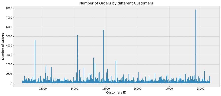
We can observe that the highest number of orders is above 7000.
To get the money spent by different customers, we use the groupby() function to highlight the customers with the highest spent amount:
#Using groupby function to highlight the Customers with highest spent amount (invoices)
money = dataset1.groupby(by=['CustomerID','Country'], as_index=False)['Amount'].sum()
print('The TOP 5 profitable customers with highest money spent...')
money.sort_values(by='Amount', ascending=False).head()
The TOP 5 profitable customers with highest money spent...
╔══════╤════════════╤════════════════╤═══════════╗
║ │ CustomerID │ Country │ Amount ║
╠══════╪════════════╪════════════════╪═══════════╣
║ 1698 │ 14646.0 │ Netherlands │ 280206.02 ║
╟──────┼────────────┼────────────────┼───────────╢
║ 4210 │ 18102.0 │ United Kingdom │ 259657.30 ║
╟──────┼────────────┼────────────────┼───────────╢
║ 3737 │ 17450.0 │ United Kingdom │ 194550.79 ║
╟──────┼────────────┼────────────────┼───────────╢
║ 3017 │ 16446.0 │ United Kingdom │ 168472.50 ║
╟──────┼────────────┼────────────────┼───────────╢
║ 1888 │ 14911.0 │ EIRE │ 143825.06 ║
╚══════╧════════════╧════════════════╧═══════════╝The below code will help us to display the money spent by different customers:
# Creating a subplot of size 15*6
plt.subplots(figsize=(15,6))
# X axis will denote the customer ID, Y axis will denote the amount spent
plt.plot(money.CustomerID, money.Amount)
plt.style.use('bmh')
plt.xlabel('Customers ID')
plt.ylabel('Money spent')
plt.title('Money Spent by different Customers')
plt.show()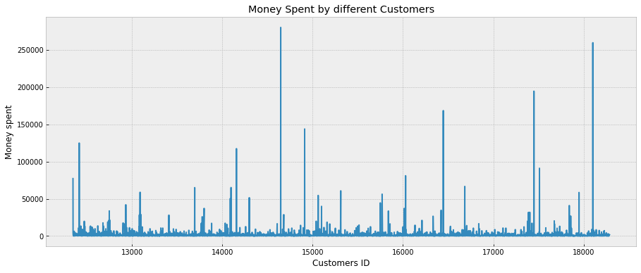
Patterns Based on Date and Time
This segment will answer the following questions:
- In which month the number of orders placed is the highest?
- On which day of the week the number of orders placed is the highest?
- At what time of the day is the store the busiest?
To answer the above questions, let's do some feature engineering. Firstly, we convert the InvoiceDate column to a datetime column.
After that, we add year_month, month, day, and hour columns:
# Convert InvoiceDate from object to datetime
dataset1['InvoiceDate'] = pd.to_datetime(dataset.InvoiceDate, format='%m/%d/%Y %H:%M')
# Creating a new feature called year_month, such that December 2010 will be denoted as 201012
dataset1.insert(loc=2, column='year_month', value=dataset1['InvoiceDate'].map(lambda x: 100*x.year + x.month))
# Creating a new feature for Month
dataset1.insert(loc=3, column='month', value=dataset1.InvoiceDate.dt.month)
# Creating a new feature for Day
# +1 to make Monday=1.....until Sunday=7
dataset1.insert(loc=4, column='day', value=(dataset1.InvoiceDate.dt.dayofweek)+1)
# Creating a new feature for Hour
dataset1.insert(loc=5, column='hour', value=dataset1.InvoiceDate.dt.hour)
Let's plot the number of orders per month:
plt.style.use('bmh')
# Using groupby to extract No. of Invoices year-monthwise
ax = dataset1.groupby('InvoiceNo')['year_month'].unique().value_counts().sort_index().plot(kind='bar',figsize=(15,6))
ax.set_xlabel('Month',fontsize=15)
ax.set_ylabel('Number of Orders',fontsize=15)
ax.set_title('Number of orders for different Months (Dec 2010 - Dec 2011)',fontsize=15)
# Providing with X tick labels
ax.set_xticklabels(('Dec_10','Jan_11','Feb_11','Mar_11','Apr_11','May_11','Jun_11','July_11','Aug_11','Sep_11','Oct_11','Nov_11','Dec_11'), rotation='horizontal', fontsize=13)
plt.show()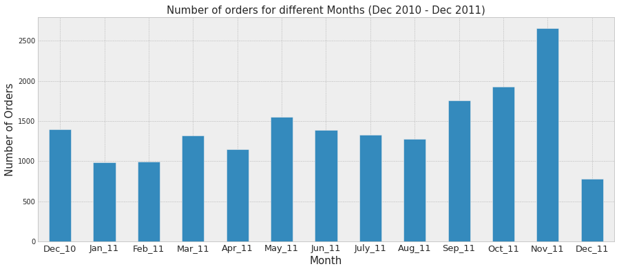
The number of orders per day:
# Day = 6 is Saturday.no orders placed
dataset1[dataset1['day']==6]
InvoiceNo StockCode year_month month day hour Description Quantity InvoiceDate UnitPrice CustomerID Country AmountWe use the groupby() function to count the number of invoices per day:
# Using groupby to count no. of Invoices daywise
ax = dataset1.groupby('InvoiceNo')['day'].unique().value_counts().sort_index().plot(kind='bar',figsize=(15,6))
ax.set_xlabel('Day', fontsize=15)
ax.set_ylabel('Number of Orders', fontsize=15)
# Giving suitable title to the plot
ax.set_title('Number of orders for different Days', fontsize=15)
# Since there are no orders placed on Saturdays, we are excluding Sat from xticklabels
ax.set_xticklabels(('Mon','Tue','Wed','Thur','Fri','Sun'), rotation='horizontal', fontsize=15)
plt.show()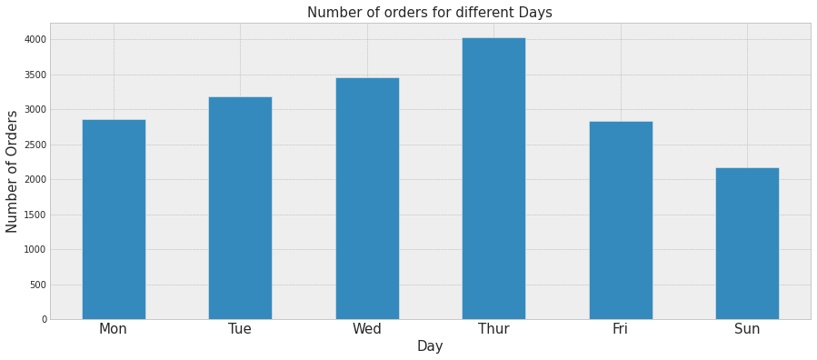
From the above plot, we view the number of orders per day except for Saturday. The highest number of orders is on Thursday.
The number of orders per hour:
# Using groupby to count the no. of Invoices hourwise
ax = dataset1.groupby('InvoiceNo')['hour'].unique().value_counts().iloc[:-2].sort_index().plot(kind='bar',figsize=(15,6))
ax.set_xlabel('Hour',fontsize=15)
ax.set_ylabel('Number of Orders',fontsize=15)
ax.set_title('Number of orders for different Hours',fontsize=15)
# Providing with X tick lables ( all orders are placed between 6 and 20 hour )
ax.set_xticklabels(range(6,21), rotation='horizontal', fontsize=15)
plt.show()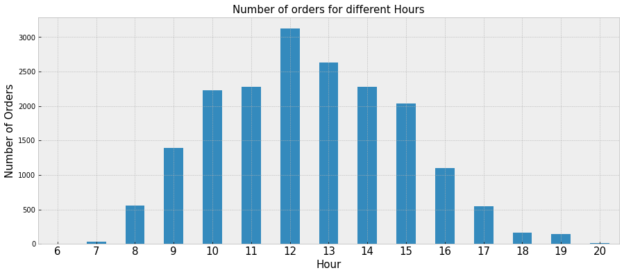
Free Items and Sales
This section will show how free products affect order volume and how discounts and incentives affect sales:
dataset1.UnitPrice.describe()count 397924.000000
mean 3.116174
std 22.096788
min 0.000000
25% 1.250000
50% 1.950000
75% 3.750000
max 8142.750000
Name: UnitPrice, dtype: float64With a minimum unit price equal to 0, there can be either some incorrect entry or free products:
# checking the distribution of unit price
plt.subplots(figsize=(12,6))
# Using darkgrid style for better visualization
sns.set_style('darkgrid')
# Applying boxplot visualization on Unit Price
sns.boxplot(dataset1.UnitPrice)
plt.show()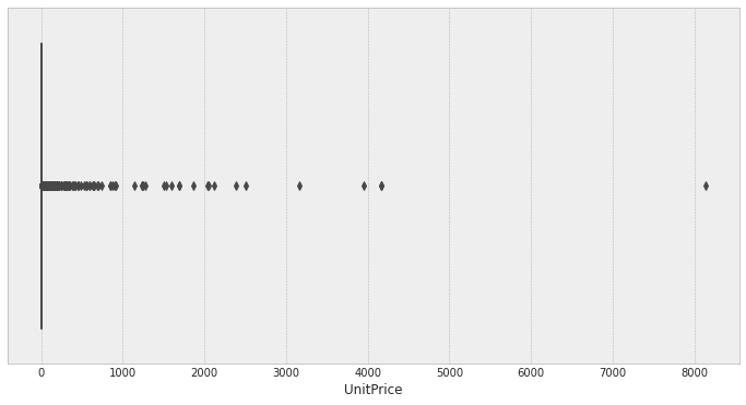
Items with UnitPrice of 0 are not outliers; these are the free items.
We will create a new dataframe of free products:
# Creating a new df of free items
freeproducts = dataset1[dataset1['UnitPrice'] == 0]
freeproducts.head()
╔═══════╤═══════════╤═══════════╤════════════╤═══════╤═════╤══════╤══════════════════════════════╤══════════╤═════════════════════╤═══════════╤════════════╤════════════════╤════════╗
║ │ InvoiceNo │ StockCode │ year_month │ month │ day │ hour │ Description │ Quantity │ InvoiceDate │ UnitPrice │ CustomerID │ Country │ Amount ║
╠═══════╪═══════════╪═══════════╪════════════╪═══════╪═════╪══════╪══════════════════════════════╪══════════╪═════════════════════╪═══════════╪════════════╪════════════════╪════════╣
║ 9302 │ 537197 │ 22841 │ 201012 │ 12 │ 7 │ 14 │ ROUND CAKE TIN VINTAGE GREEN │ 1 │ 2010-12-05 14:02:00 │ 0.0 │ 12647.0 │ Germany │ 0.0 ║
╟───────┼───────────┼───────────┼────────────┼───────┼─────┼──────┼──────────────────────────────┼──────────┼─────────────────────┼───────────┼────────────┼────────────────┼────────╢
║ 33576 │ 539263 │ 22580 │ 201012 │ 12 │ 4 │ 14 │ ADVENT CALENDAR GINGHAM SACK │ 4 │ 2010-12-16 14:36:00 │ 0.0 │ 16560.0 │ United Kingdom │ 0.0 ║
╟───────┼───────────┼───────────┼────────────┼───────┼─────┼──────┼──────────────────────────────┼──────────┼─────────────────────┼───────────┼────────────┼────────────────┼────────╢
║ 40089 │ 539722 │ 22423 │ 201012 │ 12 │ 2 │ 13 │ REGENCY CAKESTAND 3 TIER │ 10 │ 2010-12-21 13:45:00 │ 0.0 │ 14911.0 │ EIRE │ 0.0 ║
╟───────┼───────────┼───────────┼────────────┼───────┼─────┼──────┼──────────────────────────────┼──────────┼─────────────────────┼───────────┼────────────┼────────────────┼────────╢
║ 47068 │ 540372 │ 22090 │ 201012 │ 1 │ 4 │ 16 │ PAPER BUNTING RETROSPOT │ 24 │ 2011-01-06 16:41:00 │ 0.0 │ 13081.0 │ United Kingdom │ 0.0 ║
╟───────┼───────────┼───────────┼────────────┼───────┼─────┼──────┼──────────────────────────────┼──────────┼─────────────────────┼───────────┼────────────┼────────────────┼────────╢
║ 47070 │ 540372 │ 22553 │ 201012 │ 1 │ 4 │ 16 │ PLASTERS IN TIN SKULLS │ 24 │ 2011-01-06 16:41:00 │ 0.0 │ 13081.0 │ United Kingdom │ 0.0 ║
╚═══════╧═══════════╧═══════════╧════════════╧═══════╧═════╧══════╧══════════════════════════════╧══════════╧═════════════════════╧═══════════╧════════════╧════════════════╧════════╝
Let's have a view of the number of free items that were given out year-month wise:
# Counting how many free items were given out year-month wise
freeproducts.year_month.value_counts().sort_index()
201012 3
201101 3
201102 1
201103 2
201104 2
201105 2
201107 2
201108 6
201109 2
201110 3
201111 14
Name: year_month, dtype: int64We can see that there is at least one free item every month except June 2011.
Let's see the frequency of free items for different months:
# Counting how many free items were given out year-month wise
ax = freeproducts.year_month.value_counts().sort_index().plot(kind='bar',figsize=(12,6))
ax.set_xlabel('Month',fontsize=15)
ax.set_ylabel('Frequency',fontsize=15)
ax.set_title('Frequency for different Months (Dec 2010 - Dec 2011)',fontsize=15)
# Since there are 0 free items in June 2011, we are excluding it
ax.set_xticklabels(('Dec_10','Jan_11','Feb_11','Mar_11','Apr_11','May_11','July_11','Aug_11','Sep_11','Oct_11','Nov_11'), rotation='horizontal', fontsize=13)
plt.show()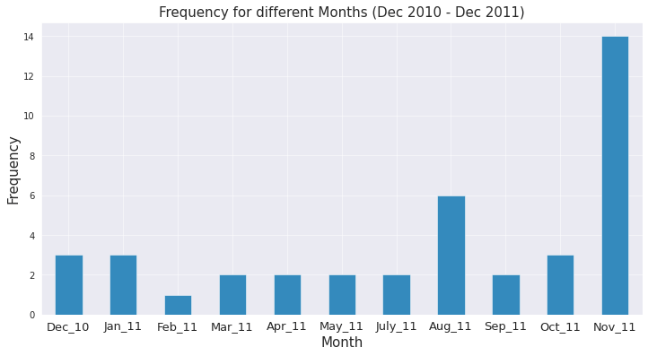
November 2011 has the most freebies. Also, compared to May, sales declined, which means there was a slight effect of nonfree items on the number of orders.
Let's get the revenue generated for different months:
plt.style.use('bmh')
# Using groupby to sum the amount spent year-month wise
ax = dataset1.groupby('year_month')['Amount'].sum().sort_index().plot(kind='bar',figsize=(15,6))
ax.set_xlabel('Month',fontsize=15)
ax.set_ylabel('Amount',fontsize=15)
ax.set_title('Revenue Generated for different Months (Dec 2010 - Dec 2011)',fontsize=15)
ax.set_xticklabels(('Dec_10','Jan_11','Feb_11','Mar_11','Apr_11','May_11','Jun_11','July_11','Aug_11','Sep_11','Oct_11','Nov_11','Dec_11'), rotation='horizontal', fontsize=13)
plt.show()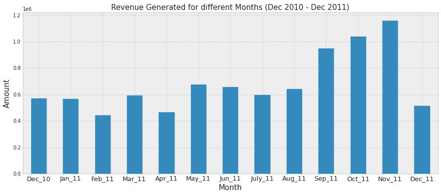
Items Insights
This segment will answer the following questions:
- Which item is bought by most of the customers?
- Which is the most sold item based on the sum of sales?
- Which is the most sold item based on the count of orders?
- Which items are the first choice items for most no. of invoices?
Most sold items based on quantity:
# Creating a new pivot table which sums the Quantity ordered for each item
most_sold= dataset1.pivot_table(index=['StockCode','Description'], values='Quantity', aggfunc='sum').sort_values(by='Quantity', ascending=False)
most_sold.reset_index(inplace=True)
sns.set_style('white')
# Creating a bar plot of Description ( or the item ) on the Y axis and the sum of Quantity on the X axis
# We are plotting only the 10 most ordered items
sns.barplot(y='Description', x='Quantity', data=most_sold.head(10))
plt.title('Top 10 Items based on No. of Sales', fontsize=14)
plt.ylabel('Item')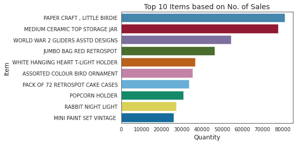
From the above plot, we can view the top 10 items based on the number of sales.
We will examine how many items were bought by the most number of customers:
# choosing WHITE HANGING HEART T-LIGHT HOLDER as a sample
d_white = dataset1[dataset1['Description']=='WHITE HANGING HEART T-LIGHT HOLDER']
# WHITE HANGING HEART T-LIGHT HOLDER has been ordered 2028 times
d_white.shape(2028, 13)# WHITE HANGING HEART T-LIGHT HOLDER has been ordered by 856 customers
len(d_white.CustomerID.unique())856# Creating a pivot table that displays the sum of unique Customers who bought particular item
most_customers = dataset1.pivot_table(index=['StockCode','Description'], values='CustomerID', aggfunc=lambda x: len(x.unique())).sort_values(by='CustomerID', ascending=False)
most_customers
# Since the count for WHITE HANGING HEART T-LIGHT HOLDER matches above length 856, the pivot table looks correct for all items╔═══════════╤════════════════════════════════════╤════════════╗
║ StockCode │ Description │ CustomerID ║
╠═══════════╪════════════════════════════════════╪════════════╣
║ 22423 │ REGENCY CAKESTAND 3 TIER │ 881 ║
╟───────────┼────────────────────────────────────┼────────────╢
║ 85123A │ WHITE HANGING HEART T-LIGHT HOLDER │ 856 ║
╟───────────┼────────────────────────────────────┼────────────╢
║ 47566 │ PARTY BUNTING │ 708 ║
╟───────────┼────────────────────────────────────┼────────────╢
║ 84879 │ ASSORTED COLOUR BIRD ORNAMENT │ 678 ║
╟───────────┼────────────────────────────────────┼────────────╢
║ 22720 │ SET OF 3 CAKE TINS PANTRY DESIGN │ 640 ║
╟───────────┼────────────────────────────────────┼────────────╢
║ ... │ ... │ ... ║
╟───────────┼────────────────────────────────────┼────────────╢
║ 21897 │ POTTING SHED CANDLE CITRONELLA │ 1 ║
╟───────────┼────────────────────────────────────┼────────────╢
║ 84795C │ OCEAN STRIPE HAMMOCK │ 1 ║
╟───────────┼────────────────────────────────────┼────────────╢
║ 90125E │ AMBER BERTIE GLASS BEAD BAG CHARM │ 1 ║
╟───────────┼────────────────────────────────────┼────────────╢
║ 90128B │ BLUE LEAVES AND BEADS PHONE CHARM │ 1 ║
╟───────────┼────────────────────────────────────┼────────────╢
║ 71143 │ SILVER BOOK MARK WITH BEADS │ 1 ║
╚═══════════╧════════════════════════════════════╧════════════╝
3897 rows × 1 columnsmost_customers.reset_index(inplace=True)
sns.set_style('white')
# Creating a bar plot of Description ( or the item ) on the Y axis and the sum of unique Customers on the X axis
# We are plotting only the 10 most bought items
sns.barplot(y='Description', x='CustomerID', data=most_customers.head(10))
# Giving suitable title to the plot
plt.title('Top 10 Items bought by Most no. of Customers', fontsize=14)
plt.ylabel('Item')
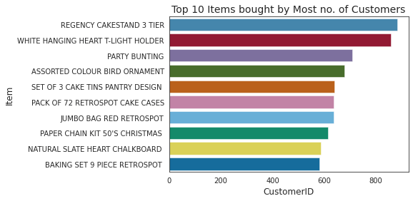
From the above plot, we can view the top items bought by the most number of customers.
Let's define our ten first choices of items:
dataset1['items'] = dataset1['Description'].str.replace(' ', '_')
# Storing all the invoice numbers into a list y
y = dataset1['InvoiceNo']
y = y.to_list()
# Using set function to find unique invoice numbers only and storing them in invoices list
invoices = list(set(y))
# Creating empty list first_choices
firstchoices = []
# looping into list of unique invoice numbers
for i in invoices:
    # the first item (index = 0) of every invoice is the first purchase
    # extracting the item name for the first purchase
    firstpurchase = dataset1[dataset1['InvoiceNo']==i]['items'].reset_index(drop=True)[0]
    # Appending the first purchase name into first choices list
    firstchoices.append(firstpurchase)
firstchoices[:5]
['LANDMARK_FRAME_CAMDEN_TOWN_',
'SET_OF_4_PANTRY_JELLY_MOULDS',
'INFLATABLE_POLITICAL_GLOBE_',
'BOUDOIR_SQUARE_TISSUE_BOX',
'EGG_CUP_HENRIETTA_HEN_CREAM_']Now, we will count repeating first choices:
# Using counter to count repeating first choices
count = Counter(firstchoices)
# Storing the counter into a datafrane
data_first_choices = pd.DataFrame.from_dict(count, orient='index').reset_index()
# Rename columns as item and count
data_first_choices.rename(columns={'index':'item', 0:'count'},inplace=True)
# Sorting the data based on count
data_first_choices.sort_values(by='count',ascending=False)
╔══════╤════════════════════════════════════╤═══════╗
║ │ item │ count ║
╠══════╪════════════════════════════════════╪═══════╣
║ 2 │ REGENCY_CAKESTAND_3_TIER │ 203 ║
╟──────┼────────────────────────────────────┼───────╢
║ 143 │ WHITE_HANGING_HEART_T-LIGHT_HOLDER │ 181 ║
╟──────┼────────────────────────────────────┼───────╢
║ 164 │ RABBIT_NIGHT_LIGHT │ 155 ║
╟──────┼────────────────────────────────────┼───────╢
║ 75 │ PARTY_BUNTING │ 122 ║
╟──────┼────────────────────────────────────┼───────╢
║ 184 │ Manual │ 119 ║
╟──────┼────────────────────────────────────┼───────╢
║ ... │ ... │ ... ║
╟──────┼────────────────────────────────────┼───────╢
║ 2133 │ SILVER_FABRIC_MIRROR │ 1 ║
╟──────┼────────────────────────────────────┼───────╢
║ 2134 │ VEGETABLE_MAGNETIC__SHOPPING_LIST │ 1 ║
╟──────┼────────────────────────────────────┼───────╢
║ 1158 │ VEGETABLE_GARDEN_CHOPPING_BOARD │ 1 ║
╟──────┼────────────────────────────────────┼───────╢
║ 2140 │ PINK_CHERRY_LIGHTS │ 1 ║
╟──────┼────────────────────────────────────┼───────╢
║ 2634 │ WALL_ART_LOVES'_SECRET_ │ 1 ║
╚══════╧════════════════════════════════════╧═══════╝We can display our ten first choices of product.
plt.subplots(figsize=(20,10))
sns.set_style('white')
# Creating a bar plot that displays Item name on the Y axis and Count on the X axis
sns.barplot(y='item', x='count', data=data_first_choices.sort_values(by='count',ascending=False).head(10))
# Giving suitable title to the plot
plt.title('Top 10 First Choices', fontsize=14)
plt.ylabel('Item')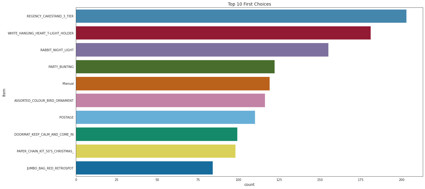
Frequently Bought Together
Market basket analysis can be defined as a data mining approach. Businesses employ it to enhance sales by understanding client purchase habits better. It includes evaluating massive data sets, such as purchase history, to uncover product groups and products likely to be purchased together.
This section will answer the question:
- Which items are frequently bought together?
We will use the groupby() function to create a basket that specifies if an item is present in a particular invoice number.
We will get the quantity present in the specific invoice number, which must be fixed.
Note that this is for all items and invoices:
basket = (dataset1.groupby(['InvoiceNo', 'Description'])['Quantity'].sum().unstack().reset_index().fillna(0).set_index('InvoiceNo'))
basket.head(5)
╔═════════════╤═══════════════════════════════╤═══════════════════════════════╤═══════════════════╤═════════════════════════════╤═════════════════════════════╤═════════════════════════╤═══════════════════════════╤═════════════════════════╤════════════════════════════════╤════════════════════════╤═════╤══════════════════════════╤═══════════════════════════╤══════════════════════════════════╤════════════════════════════════╤═════════════════════════════════╤═════════════════════════════════╤══════════════════════════════╤═════════════════════════════════╤═════════════════════════════╤══════════════════════════════════╗
║ Description │ 4 PURPLE FLOCK DINNER CANDLES │ 50'S CHRISTMAS GIFT BAG LARGE │ DOLLY GIRL BEAKER │ I LOVE LONDON MINI BACKPACK │ I LOVE LONDON MINI RUCKSACK │ NINE DRAWER OFFICE TIDY │ OVAL WALL MIRROR DIAMANTE │ RED SPOT GIFT BAG LARGE │ SET 2 TEA TOWELS I LOVE LONDON │ SPACEBOY BABY GIFT SET │ ... │ ZINC STAR T-LIGHT HOLDER │ ZINC SWEETHEART SOAP DISH │ ZINC SWEETHEART WIRE LETTER RACK │ ZINC T-LIGHT HOLDER STAR LARGE │ ZINC T-LIGHT HOLDER STARS LARGE │ ZINC T-LIGHT HOLDER STARS SMALL │ ZINC TOP 2 DOOR WOODEN SHELF │ ZINC WILLIE WINKIE CANDLE STICK │ ZINC WIRE KITCHEN ORGANISER │ ZINC WIRE SWEETHEART LETTER TRAY ║
╠═════════════╪═══════════════════════════════╪═══════════════════════════════╪═══════════════════╪═════════════════════════════╪═════════════════════════════╪═════════════════════════╪═══════════════════════════╪═════════════════════════╪════════════════════════════════╪════════════════════════╪═════╪══════════════════════════╪═══════════════════════════╪══════════════════════════════════╪════════════════════════════════╪═════════════════════════════════╪═════════════════════════════════╪══════════════════════════════╪═════════════════════════════════╪═════════════════════════════╪══════════════════════════════════╣
║ InvoiceNo │ │ │ │ │ │ │ │ │ │ │ │ │ │ │ │ │ │ │ │ │ ║
╟─────────────┼───────────────────────────────┼───────────────────────────────┼───────────────────┼─────────────────────────────┼─────────────────────────────┼─────────────────────────┼───────────────────────────┼─────────────────────────┼────────────────────────────────┼────────────────────────┼─────┼──────────────────────────┼───────────────────────────┼──────────────────────────────────┼────────────────────────────────┼─────────────────────────────────┼─────────────────────────────────┼──────────────────────────────┼─────────────────────────────────┼─────────────────────────────┼──────────────────────────────────╢
║ 536365 │ 0.0 │ 0.0 │ 0.0 │ 0.0 │ 0.0 │ 0.0 │ 0.0 │ 0.0 │ 0.0 │ 0.0 │ ... │ 0.0 │ 0.0 │ 0.0 │ 0.0 │ 0.0 │ 0.0 │ 0.0 │ 0.0 │ 0.0 │ ║
╟─────────────┼───────────────────────────────┼───────────────────────────────┼───────────────────┼─────────────────────────────┼─────────────────────────────┼─────────────────────────┼───────────────────────────┼─────────────────────────┼────────────────────────────────┼────────────────────────┼─────┼──────────────────────────┼───────────────────────────┼──────────────────────────────────┼────────────────────────────────┼─────────────────────────────────┼─────────────────────────────────┼──────────────────────────────┼─────────────────────────────────┼─────────────────────────────┼──────────────────────────────────╢
║ 536366 │ 0.0 │ 0.0 │ 0.0 │ 0.0 │ 0.0 │ 0.0 │ 0.0 │ 0.0 │ 0.0 │ 0.0 │ ... │ 0.0 │ 0.0 │ 0.0 │ 0.0 │ 0.0 │ 0.0 │ 0.0 │ 0.0 │ 0.0 │ ║
╟─────────────┼───────────────────────────────┼───────────────────────────────┼───────────────────┼─────────────────────────────┼─────────────────────────────┼─────────────────────────┼───────────────────────────┼─────────────────────────┼────────────────────────────────┼────────────────────────┼─────┼──────────────────────────┼───────────────────────────┼──────────────────────────────────┼────────────────────────────────┼─────────────────────────────────┼─────────────────────────────────┼──────────────────────────────┼─────────────────────────────────┼─────────────────────────────┼──────────────────────────────────╢
║ 536367 │ 0.0 │ 0.0 │ 0.0 │ 0.0 │ 0.0 │ 0.0 │ 0.0 │ 0.0 │ 0.0 │ 0.0 │ ... │ 0.0 │ 0.0 │ 0.0 │ 0.0 │ 0.0 │ 0.0 │ 0.0 │ 0.0 │ 0.0 │ ║
╟─────────────┼───────────────────────────────┼───────────────────────────────┼───────────────────┼─────────────────────────────┼─────────────────────────────┼─────────────────────────┼───────────────────────────┼─────────────────────────┼────────────────────────────────┼────────────────────────┼─────┼──────────────────────────┼───────────────────────────┼──────────────────────────────────┼────────────────────────────────┼─────────────────────────────────┼─────────────────────────────────┼──────────────────────────────┼─────────────────────────────────┼─────────────────────────────┼──────────────────────────────────╢
║ 536368 │ 0.0 │ 0.0 │ 0.0 │ 0.0 │ 0.0 │ 0.0 │ 0.0 │ 0.0 │ 0.0 │ 0.0 │ ... │ 0.0 │ 0.0 │ 0.0 │ 0.0 │ 0.0 │ 0.0 │ 0.0 │ 0.0 │ 0.0 │ ║
╟─────────────┼───────────────────────────────┼───────────────────────────────┼───────────────────┼─────────────────────────────┼─────────────────────────────┼─────────────────────────┼───────────────────────────┼─────────────────────────┼────────────────────────────────┼────────────────────────┼─────┼──────────────────────────┼───────────────────────────┼──────────────────────────────────┼────────────────────────────────┼─────────────────────────────────┼─────────────────────────────────┼──────────────────────────────┼─────────────────────────────────┼─────────────────────────────┼──────────────────────────────────╢
║ 536369 │ 0.0 │ 0.0 │ 0.0 │ 0.0 │ 0.0 │ 0.0 │ 0.0 │ 0.0 │ 0.0 │ 0.0 │ ... │ 0.0 │ 0.0 │ 0.0 │ 0.0 │ 0.0 │ 0.0 │ 0.0 │ 0.0 │ 0.0 │ ║
╚═════════════╧═══════════════════════════════╧═══════════════════════════════╧═══════════════════╧═════════════════════════════╧═════════════════════════════╧═════════════════════════╧═══════════════════════════╧═════════════════════════╧════════════════════════════════╧════════════════════════╧═════╧══════════════════════════╧═══════════════════════════╧══════════════════════════════════╧════════════════════════════════╧═════════════════════════════════╧═════════════════════════════════╧══════════════════════════════╧═════════════════════════════════╧═════════════════════════════╧══════════════════════════════════╝We want to know if that particular item is purchased or not. So, we encode units as 1 if purchased or 0 if not.
def encode_u(x):
  if x < 1:
    return 0
  else:
    return 1

# everything is encoded into 0 and 1
basket = basket.applymap(encode_u)
basket.head(5)
╔═════════════╤═══════════════════════════════╤═══════════════════════════════╤═══════════════════╤═════════════════════════════╤═════════════════════════════╤═════════════════════════╤═══════════════════════════╤═════════════════════════╤════════════════════════════════╤════════════════════════╤═════╤══════════════════════════╤═══════════════════════════╤══════════════════════════════════╤════════════════════════════════╤═════════════════════════════════╤═════════════════════════════════╤══════════════════════════════╤═════════════════════════════════╤═════════════════════════════╗
║ Description │ 4 PURPLE FLOCK DINNER CANDLES │ 50'S CHRISTMAS GIFT BAG LARGE │ DOLLY GIRL BEAKER │ I LOVE LONDON MINI BACKPACK │ I LOVE LONDON MINI RUCKSACK │ NINE DRAWER OFFICE TIDY │ OVAL WALL MIRROR DIAMANTE │ RED SPOT GIFT BAG LARGE │ SET 2 TEA TOWELS I LOVE LONDON │ SPACEBOY BABY GIFT SET │ ... │ ZINC STAR T-LIGHT HOLDER │ ZINC SWEETHEART SOAP DISH │ ZINC SWEETHEART WIRE LETTER RACK │ ZINC T-LIGHT HOLDER STAR LARGE │ ZINC T-LIGHT HOLDER STARS LARGE │ ZINC T-LIGHT HOLDER STARS SMALL │ ZINC TOP 2 DOOR WOODEN SHELF │ ZINC WILLIE WINKIE CANDLE STICK │ ZINC WIRE KITCHEN ORGANISER ║
╠═════════════╪═══════════════════════════════╪═══════════════════════════════╪═══════════════════╪═════════════════════════════╪═════════════════════════════╪═════════════════════════╪═══════════════════════════╪═════════════════════════╪════════════════════════════════╪════════════════════════╪═════╪══════════════════════════╪═══════════════════════════╪══════════════════════════════════╪════════════════════════════════╪═════════════════════════════════╪═════════════════════════════════╪══════════════════════════════╪═════════════════════════════════╪═════════════════════════════╣
║ InvoiceNo │ │ │ │ │ │ │ │ │ │ │ │ │ │ │ │ │ │ │ │ ║
╟─────────────┼───────────────────────────────┼───────────────────────────────┼───────────────────┼─────────────────────────────┼─────────────────────────────┼─────────────────────────┼───────────────────────────┼─────────────────────────┼────────────────────────────────┼────────────────────────┼─────┼──────────────────────────┼───────────────────────────┼──────────────────────────────────┼────────────────────────────────┼─────────────────────────────────┼─────────────────────────────────┼──────────────────────────────┼─────────────────────────────────┼─────────────────────────────╢
║ 536365 │ 0.0 │ 0.0 │ 0.0 │ 0.0 │ 0.0 │ 0.0 │ 0.0 │ 0.0 │ 0.0 │ 0.0 │ ... │ 0.0 │ 0.0 │ 0.0 │ 0.0 │ 0.0 │ 0.0 │ 0.0 │ 0.0 │ 0.0 ║
╟─────────────┼───────────────────────────────┼───────────────────────────────┼───────────────────┼─────────────────────────────┼─────────────────────────────┼─────────────────────────┼───────────────────────────┼─────────────────────────┼────────────────────────────────┼────────────────────────┼─────┼──────────────────────────┼───────────────────────────┼──────────────────────────────────┼────────────────────────────────┼─────────────────────────────────┼─────────────────────────────────┼──────────────────────────────┼─────────────────────────────────┼─────────────────────────────╢
║ 536366 │ 0.0 │ 0.0 │ 0.0 │ 0.0 │ 0.0 │ 0.0 │ 0.0 │ 0.0 │ 0.0 │ 0.0 │ ... │ 0.0 │ 0.0 │ 0.0 │ 0.0 │ 0.0 │ 0.0 │ 0.0 │ 0.0 │ 0.0 ║
╟─────────────┼───────────────────────────────┼───────────────────────────────┼───────────────────┼─────────────────────────────┼─────────────────────────────┼─────────────────────────┼───────────────────────────┼─────────────────────────┼────────────────────────────────┼────────────────────────┼─────┼──────────────────────────┼───────────────────────────┼──────────────────────────────────┼────────────────────────────────┼─────────────────────────────────┼─────────────────────────────────┼──────────────────────────────┼─────────────────────────────────┼─────────────────────────────╢
║ 536367 │ 0.0 │ 0.0 │ 0.0 │ 0.0 │ 0.0 │ 0.0 │ 0.0 │ 0.0 │ 0.0 │ 0.0 │ ... │ 0.0 │ 0.0 │ 0.0 │ 0.0 │ 0.0 │ 0.0 │ 0.0 │ 0.0 │ 0.0 ║
╟─────────────┼───────────────────────────────┼───────────────────────────────┼───────────────────┼─────────────────────────────┼─────────────────────────────┼─────────────────────────┼───────────────────────────┼─────────────────────────┼────────────────────────────────┼────────────────────────┼─────┼──────────────────────────┼───────────────────────────┼──────────────────────────────────┼────────────────────────────────┼─────────────────────────────────┼─────────────────────────────────┼──────────────────────────────┼─────────────────────────────────┼─────────────────────────────╢
║ 536368 │ 0.0 │ 0.0 │ 0.0 │ 0.0 │ 0.0 │ 0.0 │ 0.0 │ 0.0 │ 0.0 │ 0.0 │ ... │ 0.0 │ 0.0 │ 0.0 │ 0.0 │ 0.0 │ 0.0 │ 0.0 │ 0.0 │ 0.0 ║
╟─────────────┼───────────────────────────────┼───────────────────────────────┼───────────────────┼─────────────────────────────┼─────────────────────────────┼─────────────────────────┼───────────────────────────┼─────────────────────────┼────────────────────────────────┼────────────────────────┼─────┼──────────────────────────┼───────────────────────────┼──────────────────────────────────┼────────────────────────────────┼─────────────────────────────────┼─────────────────────────────────┼──────────────────────────────┼─────────────────────────────────┼─────────────────────────────╢
║ 536369 │ 0.0 │ 0.0 │ 0.0 │ 0.0 │ 0.0 │ 0.0 │ 0.0 │ 0.0 │ 0.0 │ 0.0 │ ... │ 0.0 │ 0.0 │ 0.0 │ 0.0 │ 0.0 │ 0.0 │ 0.0 │ 0.0 │ 0.0 ║
╚═════════════╧═══════════════════════════════╧═══════════════════════════════╧═══════════════════╧═════════════════════════════╧═════════════════════════════╧═════════════════════════╧═══════════════════════════╧═════════════════════════╧════════════════════════════════╧════════════════════════╧═════╧══════════════════════════╧═══════════════════════════╧══════════════════════════════════╧════════════════════════════════╧═════════════════════════════════╧═════════════════════════════════╧══════════════════════════════╧═════════════════════════════════╧═════════════════════════════╝Apriori Algorithm Concepts
Following this link, we can read this: Apriori algorithm assumes that any subset of a frequent itemset must be frequent. It's the algorithm behind Market Basket Analysis. Say, a transaction containing {Grapes, Apple, Mango} also has {Grapes, Mango}. So, according to the principle of Apriori, if {Grapes, Apple, Mango} is frequent, then {Grapes, Mango} must also be frequent.
What is Support, Confidence, Lift, and Association Rules
Support is the ratio of A-related transactions to all transactions. If out of 100 users, 10 purchase bananas, then support for bananas will be 10/100 = 10%. In other words: Support(bananas) = (Transactions involving banana)/(Total transaction).
Confidence divides the number of A and B transactions by the number of B transactions. Suppose we are looking to build a relation between bananas and tomatoes. So, if out of 40 bananas buyers, 7 buy tomatoes along with it, then confidence = 7/40 = 17.5%.
Lift is an increased sales of A when selling B; it is simply the confidence divided by the support: Lift = confidence/support. So, here lift is 17.5/10 = 1.75
Association rule mining finds interesting associations and relationships among large sets of data items. This rule shows how frequently an item set occurs in a transaction. Based on those rules created from the dataset, we perform Market Basket Analysis.
In the below program:
apriori()function returns a list of items with at least 15% support.association_rules()function returns frequent itemsets only if the level of lift score > 1(min_threshold=1).sort_values()function sorts the data frame in descending order of passed columns (lift and support).
# trying out on a sample item
wooden_star = basket.loc[basket['WOODEN STAR CHRISTMAS SCANDINAVIAN']==1]
# Using apriori algorithm, creating association rules for the sample item
# Applying apriori algorithm for wooden_star
frequentitemsets = apriori(wooden_star, min_support=0.15, use_colnames=True)
# Storing the association rules into rules
wooden_star_rules = association_rules(frequentitemsets, metric="lift", min_threshold=1)
# Sorting the rules on lift and support
wooden_star_rules.sort_values(['lift','support'],ascending=False).reset_index(drop=True)
Let's output the first four rows of the dataframe:
╔═══╤═══════════════════════════════════════════════════╤═════════════════════════════════════════╤════════════════════╤════════════════════╤══════════╤════════════╤══════════╤══════════╤════════════╗
║   │ antecedents                                       │ consequents                             │ antecedent support │ consequent support │ support  │ confidence │ lift     │ leverage │ conviction ║
╠═══╪═══════════════════════════════════════════════════╪═════════════════════════════════════════╪════════════════════╪════════════════════╪══════════╪════════════╪══════════╪══════════╪════════════╣
║ 0 │ (WOODEN TREE CHRISTMAS SCANDINAVIAN)              │ (WOODEN HEART CHRISTMAS SCANDINAVIAN)   │ 0.521940           │ 0.736721           │ 0.420323 │ 0.805310   │ 1.093101 │ 0.035799 │ 1.352299   ║
╟───┼───────────────────────────────────────────────────┼─────────────────────────────────────────┼────────────────────┼────────────────────┼──────────┼────────────┼──────────┼──────────┼────────────╢
║ 1 │ (WOODEN HEART CHRISTMAS SCANDINAVIAN)             │ (WOODEN TREE CHRISTMAS SCANDINAVIAN)    │ 0.736721           │ 0.521940           │ 0.420323 │ 0.570533   │ 1.093101 │ 0.035799 │ 1.113147   ║
╟───┼───────────────────────────────────────────────────┼─────────────────────────────────────────┼────────────────────┼────────────────────┼──────────┼────────────┼──────────┼──────────┼────────────╢
║ 2 │ (WOODEN TREE CHRISTMAS SCANDINAVIAN, WOODEN ST... │ (WOODEN HEART CHRISTMAS SCANDINAVIAN)   │ 0.521940           │ 0.736721           │ 0.420323 │ 0.805310   │ 1.093101 │ 0.035799 │ 1.352299   ║
╟───┼───────────────────────────────────────────────────┼─────────────────────────────────────────┼────────────────────┼────────────────────┼──────────┼────────────┼──────────┼──────────┼────────────╢
║ 3 │ (WOODEN HEART CHRISTMAS SCANDINAVIAN, WOODEN S... │ (WOODEN TREE CHRISTMAS SCANDINAVIAN) 	0 │ 0.736721           │ 0.521940           │ 0.420323 │ 0.570533   │ 1.093101 │ 0.035799 │ 1.113147   ║
╚═══╧═══════════════════════════════════════════════════╧═════════════════════════════════════════╧════════════════════╧════════════════════╧══════════╧════════════╧══════════╧══════════╧════════════╝
If we have a rule "B ->D", B stands for antecedent, and D stands for consequent.
Leverage is the difference between the observed frequency of B and D occurring together and the frequency that would be expected if B and D were independent.
Antecedent support computes the fraction of transactions that include the antecedent B.
Consequent support computes the support for the itemset of the consequent C.
Conviction: A high conviction value indicates that the consequent strongly depends on the antecedent.
You can refer to this link for more information.
Now, we will create the function in which we pass an item name, and it returns the items that are frequently bought together:
# In other words, it returns the items which are likely to be bought by user because he bought the item passed into function
def frequently_bought_t(item):
    # df of item passed
    item_d = basket.loc[basket[item]==1]
    # Applying apriori algorithm on item df
    frequentitemsets = apriori(item_d, min_support=0.15, use_colnames=True)
    # Storing association rules
    rules = association_rules(frequentitemsets, metric="lift", min_threshold=1)
    # Sorting on lift and support
    rules.sort_values(['lift','support'],ascending=False).reset_index(drop=True)
    print('Items frequently bought together with {0}'.format(item))
    # Returning top 6 items with highest lift and support
    return rules['consequents'].unique()[:6]
frequently_bought_t('WOODEN STAR CHRISTMAS SCANDINAVIAN')Items frequently bought together with WOODEN STAR CHRISTMAS SCANDINAVIAN
array([frozenset({'WOODEN HEART CHRISTMAS SCANDINAVIAN'}),
frozenset({"PAPER CHAIN KIT 50'S CHRISTMAS "}),
frozenset({'WOODEN STAR CHRISTMAS SCANDINAVIAN'}),
frozenset({'SET OF 3 WOODEN HEART DECORATIONS'}),
frozenset({'SET OF 3 WOODEN SLEIGH DECORATIONS'}),
frozenset({'SET OF 3 WOODEN STOCKING DECORATION'})], dtype=object)frequently_bought_t('JAM MAKING SET WITH JARS')Items frequently bought together with JAM MAKING SET WITH JARS
array([frozenset({'JAM MAKING SET PRINTED'}),
frozenset({'JAM MAKING SET WITH JARS'}),
frozenset({'PACK OF 72 RETROSPOT CAKE CASES'}),
frozenset({'RECIPE BOX PANTRY YELLOW DESIGN'}),
frozenset({'REGENCY CAKESTAND 3 TIER'}),
frozenset({'SET OF 3 CAKE TINS PANTRY DESIGN '})], dtype=object)We can have a view of the items which are commonly purchased together.
Conclusion
As we have said initially, Market Basket Analysis is a method for understanding client purchase trends based on historical data. In this tutorial, we have performed EDA to understand the relationship between the customers' products, and we have introduced you to the Market Basket Analysis technique.
You can check the code for this tutorial in this Colab notebook.
Learn also: Customer Churn Prediction: A Complete Guide in Python.
Happy learning ♥
Just finished the article? Why not take your Python skills a notch higher with our Python Code Assistant? Check it out!
View Full Code Switch My Framework


Got a coding query or need some guidance before you comment? Check out this Python Code Assistant for expert advice and handy tips. It's like having a coding tutor right in your fingertips!