How to Create Plots with Plotly In Python

Step up your coding game with AI-powered Code Explainer. Get insights like never before!

Nothing is better than well designed figures to give a clearer view of reports and do accurate conclusions for them, hence the use of the visualization tools is a key thing when it comes to the exploratory data analysis step that should be undergone by data scientists.

In this tutorial, we will learn how to use Plotly visualization tool to create dynamic plots in Python. 

The development environment that we will be using throughout this tutorial is a Jupyter lab, if you don't have it installed, this link should help you install it.

Make sure you install the required libraries:

pip install numpy
pip install pandas 
pip install plotly

If you're not using Anaconda environment, then you must manually install plotly extension for jupyter lab:

$ jupyter labextension install jupyterlab-plotly

Once you have everything install, open up a new jupyter lab and import these libraries in the first cell:

import pandas as pd
import numpy as np
import plotly.offline as py
import plotly.graph_objs as go
import plotly.figure_factory as ff
import yfinance as yf
import pandas_datareader as pdr

py.init_notebook_mode()

We're running the init_notebook_mode() method to enable the use of plotly library without registering and getting an API key for that.

Simple Line Plots

To create figures using Plotly, we need to create an instance of the Figure class, the main components of this class are:

• Layout: Which is the metadata and the external information that appears to the graph like the main title and the names of the axis. We can add the layout by assigning a value to the layout attribute of the Figure object, which is an instance of the class go.Layout
• Traces: Which is a set of graphical objects Plotly offers like Scatter, Bar, Histogram plots, etc. We can add traces by calling the method add_trace() to the Figure object.

Here is a simple example of displaying the graph of the function f(x) = 2x.

x = [ i for i in range(-10,10) ]

y = [ i*2 for i in range(-10,10) ]

xaxis = go.layout.XAxis(title="X Axis")
yaxis = go.layout.YAxis(title="Y Axis")

fig = go.Figure(layout=go.Layout(title="Simple Line Plot", xaxis=xaxis, yaxis=yaxis))
fig.add_trace(go.Scatter(x=x, y=y))

Here is another example of displaying the graph of the sigmoid function (usually used as an activation function in deep learning) which is defined by the formula: s(x) = 1/ (1 + exp(-x)).

To change the color of the lines, we assign a dictionary to the marker attribute and specify color as a key and the name of the color (in our case, red) as a value.

def sigmoid(x):
    return 1 / (1 + np.exp((-1) * x))

x = sorted(np.random.random(100) * 10 - 5)
y = [ sigmoid(i) for i in x ]

xaxis = go.layout.XAxis(title="X Axis")
yaxis = go.layout.YAxis(title="Y Axis")

fig=go.Figure(layout=go.Layout(title="Sigmoid Plot",xaxis=xaxis, yaxis=yaxis))
fig.add_trace(go.Scatter(x=x, y=y, marker=dict(color="red")))

Multiple Scatter Plots 

In this section, we will learn to plot dotted type of plots (unlike continuous lines in the first section). We will try to plot 4 scatter plots within the same figure. 

To generate random data, we will use the np.random.randint() method from Numpy, we will specify the two boundaries (lowest and highest numbers) in addition to the size of the array (in our case, let's use 50).

In order to have the dotted shape format of the plot, we need to assign the attribute mode the value markers.

l = []

for _ in range(5):
    l.append([ sorted(np.random.randint(low=0, high=10000, size=50)), sorted(np.random.randint(low=0, high=10000, size=50)) ])

l = np.array(l)

figure = go.Figure(layout=go.Layout(title="Simple Scatter Example", xaxis=go.layout.XAxis(title="X"), yaxis=go.layout.YAxis(title="Y")))
for i in range(len(l)):
    figure.add_trace(go.Scatter(x=l[i][0],y=l[i][1], mode="markers", name=f" Distribution {i+1} "))
figure.show()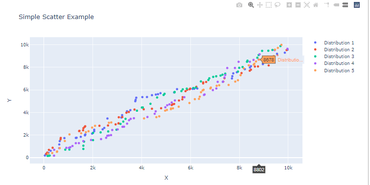

Bars And Distribution Plots

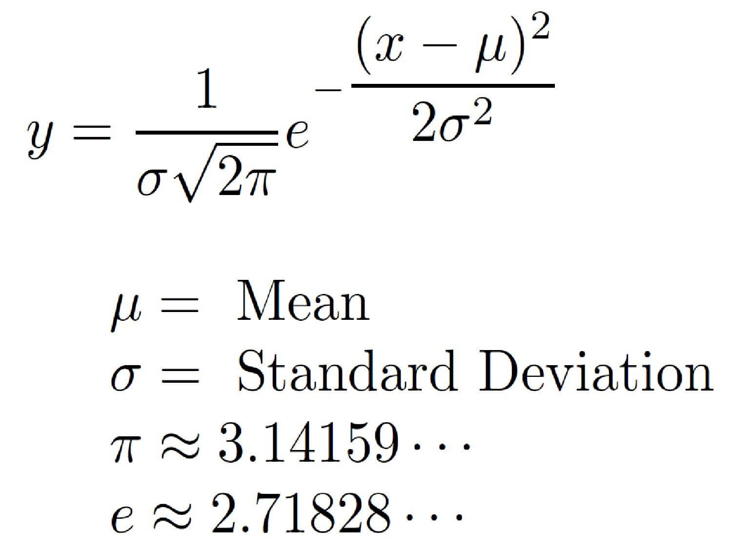
A normal (Gaussian) distribution is among the most famous statistical distributions. It is defined by two mains properties the mean μ and the standard deviation σ, from this formula:

First, we will create a simple normal distribution using Numpy with the method np.random.normal() function. Then, we will plot it as histogram with no distribution line curve.

dist = np.random.normal(loc=0, scale=1, size=50000)

figure = go.Figure()
figure.add_trace(go.Histogram(x=dist,))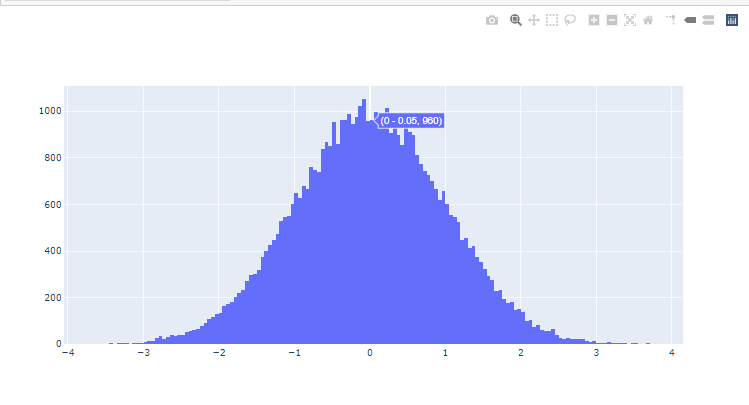

Now let us create multiple distributions, with the same mean μ=0 but by changing the standard deviation σ values. The bigger the more flattened our distribution plots will be (like shown in the figure below). 

In this case we will use the plotly.figure_factory module which offers more complex graphical objects:

d=[{"values":np.random.normal(0,0.5,10000), "information": " Normal Distribution with mean 0 and std= 0.5"},
  {"values":np.random.normal(0,1,10000), "information": " Normal Distribution with mean 0 and std= 1"},
  {"values":np.random.normal(0,1.5,10000), "information": " Normal Distribution with mean 0 and std= 1.5"},
  {"values":np.random.normal(0,2,10000), "information": " Normal Distribution with mean 0 and std= 2"},
  {"values":np.random.normal(0,5,10000), "information": " Normal Distribution with mean 0 and std= 5"}]

ff.create_distplot([ele["values"] for ele in d], group_labels=[ele["information"] for ele in d], show_hist=False)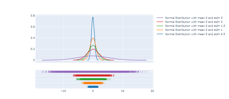

3D Scatter Plots

To create 3D Scatter plots it is also straightforward, first let us generate random array of numbers x,y and z using np.random.randint(). Then we will create a Scatter3d plot by adding it as a trace for the Figure object.

x = np.random.randint(low=5, high=100, size=15)
y = np.random.randint(low=5, high=100 ,size=15)
z = np.random.randint(low=5, high=100, size=15)

fig=go.Figure()
fig.add_trace(go.Scatter3d(x=x, y=y, z=z, mode="markers"))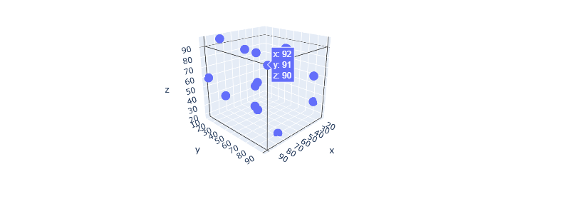

Every feature is considered a dimension in data science, the high the features the better the accuracy to classify data belonging to different labels.

We will use the Iris dataset which contains information about iris flower species; setosa, versicolor and virginica. The features available are the sepal width, sepal length, petal width and petal length. You can download the dataset here.

We will use a 3D Scatter plot to display three features (sepal width/sepal length/petal width) and label every data point to its specie type. 

In Pandas, unique().tolist() allows us to store all unique values in a Pandas serie in a list, like here we are storing the species types in a list (species_types).

fig = go.Figure()
species_types = df_iris.species.unique().tolist()

for specie in species_types:
    b = df_iris.species == specie
    fig.add_trace(go.Scatter3d(x=df_iris["sepal_length"][b], y=df_iris["sepal_width"][b], z=df_iris["petal_width"][b], name=specie, mode="markers"))

fig.show()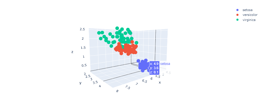

The amazing thing about this, is you can interact with the 3D plot and view different places of it.

Using Plotly for Financial Data and CandleSticks Charts

For this section, we will read stock price data of Apple and Microsoft that we will download using yfinance wrapper for Yahoo Finance API and pandas-datareader library.

If you need more depth on how you can import financial data from these libraries, I suggest you check this tutorial.

We will first use a simple line plot to compare the change of stock prices for both AAPL and MSFT by displaying their close prices respectively:

yf.pdr_override()

symbols = ["AAPL","MSFT"]
stocks = []
for symbol in symbols:
    stocks.append(pdr.get_data_yahoo(symbol, start="2020-01-01", end="2020-05-31"))

fig = go.Figure()

for stock,symbol in zip(stocks,symbols):
    fig.add_trace(go.Scatter(x=stock.index, y=stock.Close, name=symbol))

fig.show()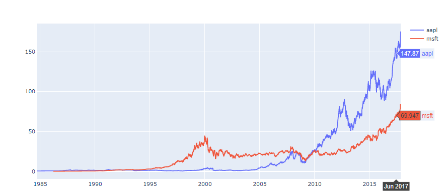

We will now use plotly.figure_factory to generate the candlestick chart. 

df_aapl = pdr.get_data_yahoo(symbol, start="2020-01-01", end="2020-05-31")
ff.create_candlestick(dates=df_aapl.index, open=df_aapl.Open, high=df_aapl.High, low=df_aapl.Low, close=df_aapl.Close)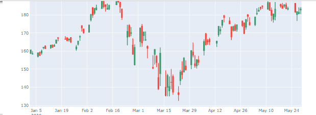

Conclusion

In this tutorial you have learned to:

• Generate numbers in numpy and pandas.
• Create different types of plots (Scatter, Histograms, etc.)
• Change the esthetics of your figures (color, marker).
• Plot statistical distributions (such as Gaussian). 
• Plot candlesticks charts.

Read also: Introduction to Finance and Technical Indicators with Python.

Please check the full notebook here.

Happy Coding ♥

Let our Code Converter simplify your multi-language projects. It's like having a coding translator at your fingertips. Don't miss out!

Read Also

Introduction to Finance and Technical Indicators with Python

Learn how to handle stock prices in Python, understand the candles prices format (OHLC), plotting them using candlestick charts as well as learning to use many technical indicators using stockstats library in Python.

How to Generate Random Data in Python

Generating random integers, floating point numbers, strings and bytes using random, os and secrets built-in modules in Python.

How to Perform Voice Gender Recognition using TensorFlow in Python

Learn how to build a deep learning model that is able to detect and recognize your gender just by your voice tone using Tensorflow framework in Python.

Comment panel