Unlock the secrets of your code with our AI-powered Code Explainer. Take a look!
Introduction
Fake news is the intentional broadcasting of false or misleading claims as news, where the statements are purposely deceitful.
Newspapers, tabloids, and magazines have been supplanted by digital news platforms, blogs, social media feeds, and a plethora of mobile news applications. News organizations benefitted from the increased use of social media and mobile platforms by providing subscribers with up-to-the-minute information.
Consumers now have instant access to the latest news. These digital media platforms have increased in prominence due to their easy connectedness to the rest of the world and allow users to discuss and share ideas and debate topics such as democracy, education, health, research, and history. Fake news items on digital platforms are getting more popular and are used for profit, such as political and financial gain.
How Big is this Problem?
Because the Internet, social media, and digital platforms are widely used, anybody may propagate inaccurate and biased information. It is almost impossible to prevent the spread of fake news. There is a tremendous surge in the distribution of false news, which is not restricted to one sector such as politics but includes sports, health, history, entertainment, and science and research.
The Solution
It is vital to recognize and differentiate between false and accurate news. One method is to have an expert decide, and fact checks every piece of information, but this takes time and needs expertise that cannot be shared. Secondly, we can use machine learning and artificial intelligence tools to automate the identification of fake news.
Online news information includes various unstructured format data (such as documents, videos, and audio), but we will concentrate on text format news here. With the progress of machine learning and Natural language processing, we can now recognize the misleading and false character of an article or statement.
Several studies and experiments are being conducted to detect fake news across all mediums.
Our main goal for this tutorial is:
- Explore and analyze the Fake News dataset.
- Build a classifier that can distinguish Fake news with as much accuracy as possible.
Here is the table of content:
- Introduction
- How Big is this Problem?
- The Solution
- Data Exploration
- Data Cleaning for Analysis
- Explorative Data Analysis
- Building a Classifier by Fine-tuning BERT
- Appendix: Creating a Submission File for Kaggle
- Conclusion
Data Exploration
In this work, we utilized the fake news dataset from Kaggle to classify untrustworthy news articles as fake news. We have a complete training dataset containing the following characteristics:
id: unique id for a news articletitle: title of a news articleauthor: author of the news articletext: text of the article; could be incompletelabel: a label that marks the article as potentially unreliable denoted by 1 (unreliable or fake) or 0 (reliable).
It is a binary classification problem in which we must predict if a particular news story is reliable or not.
If you have a Kaggle account, you can simply download the dataset from the website there and extract the ZIP file.
I also uploaded the dataset into Google Drive, and you can get it here or use the gdown library to download it in Google Colab or Jupyter notebooks automatically:
$ pip install gdown# download from Google Drive
$ gdown "https://drive.google.com/uc?id=178f_VkNxccNidap-5-uffXUW475pAuPy&confirm=t"Downloading...
From: https://drive.google.com/uc?id=178f_VkNxccNidap-5-uffXUW475pAuPy&confirm=t
To: /content/fake-news.zip
100% 48.7M/48.7M [00:00<00:00, 74.6MB/s]Unzipping the files:
$ unzip fake-news.zipThree files will appear in the current working directory: train.csv, test.csv, and submit.csv, we will be using train.csv in most of the tutorial.
Installing the required dependencies:
$ pip install transformers nltk pandas numpy matplotlib seaborn wordcloudNote: If you're in a local environment, make sure you install PyTorch for GPU, head to this page for a proper installation.
Let's import the essential libraries for analysis:
import pandas as pd
import numpy as np
import matplotlib.pyplot as plt
import seaborn as sns
The NLTK corpora and modules must be installed using the standard NLTK downloader:
import nltk
nltk.download('stopwords')
nltk.download('wordnet')
The fake news dataset comprises various authors' original and fictitious article titles and text. Let's import our dataset:
# load the dataset
news_d = pd.read_csv("train.csv")
print("Shape of News data:", news_d.shape)
print("News data columns", news_d.columns)Output:
 Shape of News data: (20800, 5)
 News data columns Index(['id', 'title', 'author', 'text', 'label'], dtype='object')
Here's how the dataset looks:
# by using df.head(), we can immediately familiarize ourselves with the dataset.
news_d.head()
Output:
id	title	author	text	label
0	0	House Dem Aide: We Didn’t Even See Comey’s Let...	Darrell Lucus	House Dem Aide: We Didn’t Even See Comey’s Let...	1
1	1	FLYNN: Hillary Clinton, Big Woman on Campus - ...	Daniel J. Flynn	Ever get the feeling your life circles the rou...	0
2	2	Why the Truth Might Get You Fired	Consortiumnews.com	Why the Truth Might Get You Fired October 29, ...	1
3	3	15 Civilians Killed In Single US Airstrike Hav...	Jessica Purkiss	Videos 15 Civilians Killed In Single US Airstr...	1
4	4	Iranian woman jailed for fictional unpublished...	Howard Portnoy	Print \nAn Iranian woman has been sentenced to...	1
We have 20,800 rows, which have five columns. Let's see some statistics of the text column:
#Text Word startistics: min.mean, max and interquartile range

txt_length = news_d.text.str.split().str.len()
txt_length.describe()
Output:
count    20761.000000
mean       760.308126
std        869.525988
min          0.000000
25%        269.000000
50%        556.000000
75%       1052.000000
max      24234.000000
Name: text, dtype: float64
Stats for the title column:
#Title statistics

title_length = news_d.title.str.split().str.len()
title_length.describe()
Output:
count    20242.000000
mean        12.420709
std          4.098735
min          1.000000
25%         10.000000
50%         13.000000
75%         15.000000
max         72.000000
Name: title, dtype: float64
The statistics for the training and testing sets are as follows:
- The
textattribute has a higher word count with an average of 760 words and 75% having more than 1000 words. - The
titleattribute is a short statement with an average of 12 words, and 75% of them are around 15 words.
Our experiment would be with both text and title together.
Distribution of Classes
Counting plots for both labels:
sns.countplot(x="label", data=news_d);
print("1: Unreliable")
print("0: Reliable")
print("Distribution of labels:")
print(news_d.label.value_counts());
Output:
1: Unreliable
0: Reliable
Distribution of labels:
1    10413
0    10387
Name: label, dtype: int64
print(round(news_d.label.value_counts(normalize=True),2)*100);Output:
1    50.0
0    50.0
Name: label, dtype: float64
The number of untrustworthy articles (fake or 1) is 10413, while the number of trustworthy articles (reliable or 0) is 10387. Almost 50% of the articles are fake. Therefore, the accuracy metric will measure how well our model is doing when building a classifier.
Data Cleaning for Analysis
In this section, we will clean our dataset to do some analysis:
- Drop unused rows and columns.
- Perform null value imputation.
- Remove special characters.
- Remove stop words.
# Constants that are used to sanitize the datasets

column_n = ['id', 'title', 'author', 'text', 'label']
remove_c = ['id','author']
categorical_features = []
target_col = ['label']
text_f = ['title', 'text']
# Clean Datasets
import nltk
from nltk.corpus import stopwords
import re
from nltk.stem.porter import PorterStemmer
from collections import Counter
ps = PorterStemmer()
wnl = nltk.stem.WordNetLemmatizer()
stop_words = stopwords.words('english')
stopwords_dict = Counter(stop_words)
# Removed unused clumns
def remove_unused_c(df,column_n=remove_c):
df = df.drop(column_n,axis=1)
return df
# Impute null values with None
def null_process(feature_df):
for col in text_f:
feature_df.loc[feature_df[col].isnull(), col] = "None"
return feature_df
def clean_dataset(df):
# remove unused column
df = remove_unused_c(df)
#impute null values
df = null_process(df)
return df
# Cleaning text from unused characters
def clean_text(text):
text = str(text).replace(r'http[\w:/\.]+', ' ') # removing urls
text = str(text).replace(r'[^\.\w\s]', ' ') # remove everything but characters and punctuation
text = str(text).replace('[^a-zA-Z]', ' ')
text = str(text).replace(r'\s\s+', ' ')
text = text.lower().strip()
#text = ' '.join(text)
return text
## Nltk Preprocessing include:
# Stop words, Stemming and Lemmetization
# For our project we use only Stop word removal
def nltk_preprocess(text):
text = clean_text(text)
wordlist = re.sub(r'[^\w\s]', '', text).split()
#text = ' '.join([word for word in wordlist if word not in stopwords_dict])
#text = [ps.stem(word) for word in wordlist if not word in stopwords_dict]
text = ' '.join([wnl.lemmatize(word) for word in wordlist if word not in stopwords_dict])
return textIn the code block above:
- We have imported NLTK, which is a famous platform for developing Python applications that interact with human language. Next, we import
refor regex. - We import stopwords from
nltk.corpus. When working with words, particularly when considering semantics, we sometimes need to eliminate common words that do not add any significant meaning to a statement, such as"but","can","we", etc. PorterStemmeris used to perform stemming words with NLTK. Stemmers strip words of their morphological affixes, leaving the word stem solely.- We import
WordNetLemmatizer()from NLTK library for lemmatization. Lemmatization is much more effective than stemming. It goes beyond word reduction and evaluates a language's whole lexicon to apply morphological analysis to words, with the goal of just removing inflectional ends and returning the base or dictionary form of a word, known as the lemma. stopwords.words('english')allow us to look at the list of all the English stop words supported by NLTK.remove_unused_c()function is used to remove the unused columns.- We impute null values with
Noneusing thenull_process()function. - Inside the function
clean_dataset(), we callremove_unused_c()andnull_process()functions. This function is responsible for data cleaning. - To clean text from unused characters, we have created the
clean_text()function. - For preprocessing, we will use only stop word removal. We created the
nltk_preprocess()function for that purpose.
Preprocessing the text and title:
# Perform data cleaning on train and test dataset by calling clean_dataset function
df = clean_dataset(news_d)
# apply preprocessing on text through apply method by calling the function nltk_preprocess
df["text"] = df.text.apply(nltk_preprocess)
# apply preprocessing on title through apply method by calling the function nltk_preprocess
df["title"] = df.title.apply(nltk_preprocess)
# Dataset after cleaning and preprocessing step
df.head()Output:
title	text	label
0	house dem aide didnt even see comeys letter ja...	house dem aide didnt even see comeys letter ja...	1
1	flynn hillary clinton big woman campus breitbart	ever get feeling life circle roundabout rather...	0
2	truth might get fired	truth might get fired october 29 2016 tension ...	1
3	15 civilian killed single u airstrike identified	video 15 civilian killed single u airstrike id...	1
4	iranian woman jailed fictional unpublished sto...	print iranian woman sentenced six year prison ...	1
Explorative Data Analysis
In this section, we will perform:
- Univariate Analysis: It is a statistical analysis of the text. We will use word cloud for that purpose. A word cloud is a visualization approach for text data where the most common term is presented in the most considerable font size.
- Bivariate Analysis: Bigram and Trigram will be used here. According to Wikipedia: "an n-gram is a contiguous sequence of n items from a given sample of text or speech. According to the application, the items can be phonemes, syllables, letters, words, or base pairs. The n-grams are typically collected from a text or speech corpus".
Single-word Cloud
The most frequent words appear in a bold and bigger font in a word cloud. This section will perform a word cloud for all words in the dataset.
The WordCloud library's wordcloud() function will be used, and the generate() is utilized for generating the word cloud image:
from wordcloud import WordCloud, STOPWORDS
import matplotlib.pyplot as plt

# initialize the word cloud
wordcloud = WordCloud( background_color='black', width=800, height=600)
# generate the word cloud by passing the corpus
text_cloud = wordcloud.generate(' '.join(df['text']))
# plotting the word cloud
plt.figure(figsize=(20,30))
plt.imshow(text_cloud)
plt.axis('off')
plt.show()
Output:
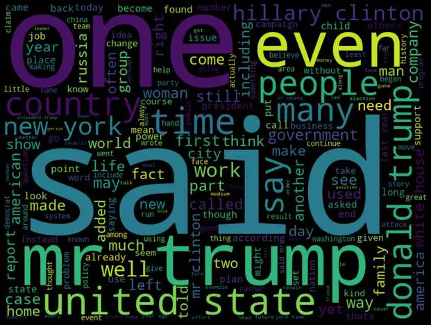
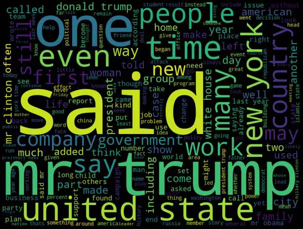
Word cloud for reliable news only:
true_n = ' '.join(df[df['label']==0]['text'])
wc = wordcloud.generate(true_n)
plt.figure(figsize=(20,30))
plt.imshow(wc)
plt.axis('off')
plt.show()
Output:
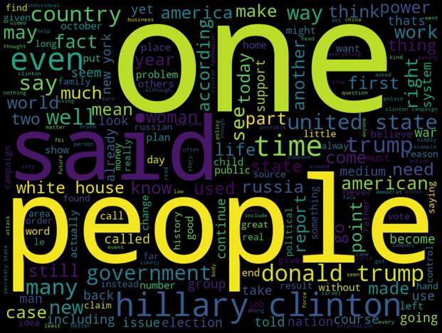
Word cloud for fake news only:
fake_n = ' '.join(df[df['label']==1]['text'])
wc= wordcloud.generate(fake_n)
plt.figure(figsize=(20,30))
plt.imshow(wc)
plt.axis('off')
plt.show()
Output:
Most Frequent Bigram (Two-word Combination)
An N-gram is a sequence of letters or words. A character unigram is made up of a single character, while a bigram comprises a series of two characters. Similarly, word N-grams are made up of a series of n words. The word "united" is a 1-gram (unigram). The combination of the words "united state" is a 2-gram (bigram), "new york city" is a 3-gram.
Let's plot the most common bigram on the reliable news:
def plot_top_ngrams(corpus, title, ylabel, xlabel="Number of Occurences", n=2):
  """Utility function to plot top n-grams"""
  true_b = (pd.Series(nltk.ngrams(corpus.split(), n)).value_counts())[:20]
  true_b.sort_values().plot.barh(color='blue', width=.9, figsize=(12, 8))
  plt.title(title)
  plt.ylabel(ylabel)
  plt.xlabel(xlabel)
  plt.show()
plot_top_ngrams(true_n, 'Top 20 Frequently Occuring True news Bigrams', "Bigram", n=2)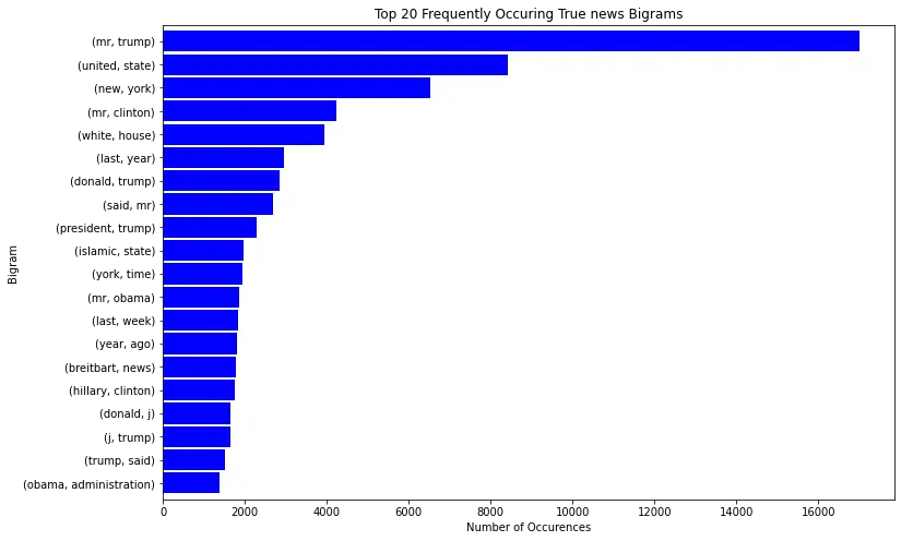
The most common bigram on the fake news:
plot_top_ngrams(fake_n, 'Top 20 Frequently Occuring Fake news Bigrams', "Bigram", n=2)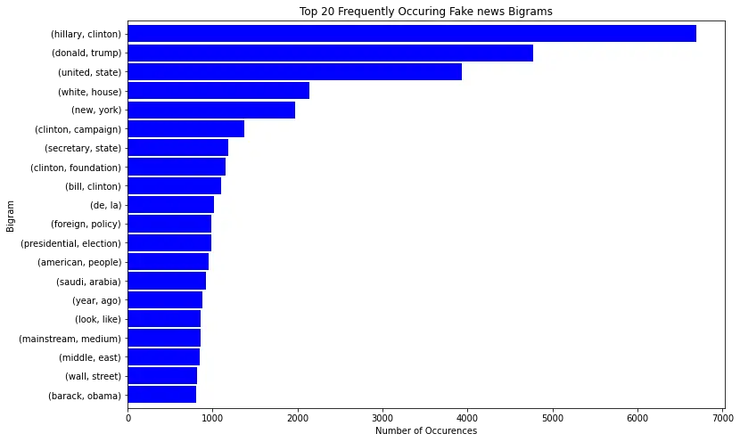
Most Frequent Trigram (Three-word combination)
The most common trigram on reliable news:
plot_top_ngrams(true_n, 'Top 20 Frequently Occuring True news Trigrams', "Trigrams", n=3)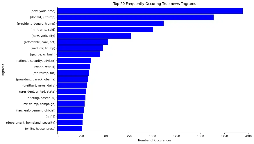
For fake news now:
plot_top_ngrams(fake_n, 'Top 20 Frequently Occuring Fake news Trigrams', "Trigrams", n=3)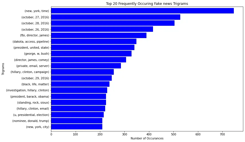
The above plots give us some ideas on how both classes look. In the next section, we'll use the transformers library to build a fake news detector.
Building a Classifier by Fine-tuning BERT
This section will be grabbing code extensively from the fine-tuning BERT tutorial to make a fake news classifier using the transformers library. So, for more detailed information, you can head to the original tutorial.
If you didn't install transformers, you have to:
$ pip install transformersLet's import the necessary libraries:
import torch
from transformers.file_utils import is_tf_available, is_torch_available, is_torch_tpu_available
from transformers import BertTokenizerFast, BertForSequenceClassification
from transformers import Trainer, TrainingArguments
import numpy as np
from sklearn.model_selection import train_test_split

import random
We want to make our results reproducible even if we restart our environment:
def set_seed(seed: int):
    """
    Helper function for reproducible behavior to set the seed in ``random``, ``numpy``, ``torch`` and/or ``tf`` (if
    installed).

    Args:
        seed (:obj:`int`): The seed to set.
    """
    random.seed(seed)
    np.random.seed(seed)
    if is_torch_available():
        torch.manual_seed(seed)
        torch.cuda.manual_seed_all(seed)
        # ^^ safe to call this function even if cuda is not available
    if is_tf_available():
        import tensorflow as tf

        tf.random.set_seed(seed)

set_seed(1)
The model we're going to use is the bert-base-uncased:
# the model we gonna train, base uncased BERT
# check text classification models here: https://huggingface.co/models?filter=text-classification
model_name = "bert-base-uncased"
# max sequence length for each document/sentence sample
max_length = 512
Loading the tokenizer:
# load the tokenizer
tokenizer = BertTokenizerFast.from_pretrained(model_name, do_lower_case=True)
Data Preparation
Let's now clean NaN values from text, author, and title columns:
news_df = news_d[news_d['text'].notna()]
news_df = news_df[news_df["author"].notna()]
news_df = news_df[news_df["title"].notna()]
Next, making a function that takes the dataset as a Pandas dataframe and returns the train/validation splits of texts and labels as lists:
def prepare_data(df, test_size=0.2, include_title=True, include_author=True):
  texts = []
  labels = []
  for i in range(len(df)):
    text = df["text"].iloc[i]
    label = df["label"].iloc[i]
    if include_title:
      text = df["title"].iloc[i] + " - " + text
    if include_author:
      text = df["author"].iloc[i] + " : " + text
    if text and label in [0, 1]:
      texts.append(text)
      labels.append(label)
  return train_test_split(texts, labels, test_size=test_size)

train_texts, valid_texts, train_labels, valid_labels = prepare_data(news_df)
The above function takes the dataset in a dataframe type and returns them as lists split into training and validation sets. Setting include_title to True means that we add the title column to the text we going to use for training, setting include_author to True means we add the author to the text as well.
Let's make sure the labels and texts have the same length:
print(len(train_texts), len(train_labels))
print(len(valid_texts), len(valid_labels))
Output:
14628 14628
3657 3657
Learn also: Fine-tuning BERT for Semantic Textual Similarity with Transformers in Python.
Tokenizing the Dataset
Let's use the BERT tokenizer to tokenize our dataset:
# tokenize the dataset, truncate when passed `max_length`,
# and pad with 0's when less than `max_length`
train_encodings = tokenizer(train_texts, truncation=True, padding=True, max_length=max_length)
valid_encodings = tokenizer(valid_texts, truncation=True, padding=True, max_length=max_length)
Converting the encodings into a PyTorch dataset:
class NewsGroupsDataset(torch.utils.data.Dataset):
    def __init__(self, encodings, labels):
        self.encodings = encodings
        self.labels = labels

    def __getitem__(self, idx):
        item = {k: torch.tensor(v[idx]) for k, v in self.encodings.items()}
        item["labels"] = torch.tensor([self.labels[idx]])
        return item

    def __len__(self):
        return len(self.labels)

# convert our tokenized data into a torch Dataset
train_dataset = NewsGroupsDataset(train_encodings, train_labels)
valid_dataset = NewsGroupsDataset(valid_encodings, valid_labels)
Loading and Fine-tuning the Model
We'll be using BertForSequenceClassification to load our BERT transformer model:
# load the model
model = BertForSequenceClassification.from_pretrained(model_name, num_labels=2)
We set num_labels to 2 since it's a binary classification. Below function is a callback to calculate the accuracy on each validation step:
from sklearn.metrics import accuracy_score

def compute_metrics(pred):
  labels = pred.label_ids
  preds = pred.predictions.argmax(-1)
  # calculate accuracy using sklearn's function
  acc = accuracy_score(labels, preds)
  return {
      'accuracy': acc,
  }
Let's initialize the training parameters:
training_args = TrainingArguments(
    output_dir='./results',          # output directory
    num_train_epochs=1,              # total number of training epochs
    per_device_train_batch_size=10,  # batch size per device during training
    per_device_eval_batch_size=20,   # batch size for evaluation
    warmup_steps=100,                # number of warmup steps for learning rate scheduler
    logging_dir='./logs',            # directory for storing logs
    load_best_model_at_end=True,     # load the best model when finished training (default metric is loss)
    # but you can specify `metric_for_best_model` argument to change to accuracy or other metric
    logging_steps=200,               # log & save weights each logging_steps
    save_steps=200,
    evaluation_strategy="steps",     # evaluate each `logging_steps`
)
I've set the per_device_train_batch_size to 10, but you should set it as high as your GPU could possibly fit. Setting the logging_steps and save_steps to 200, meaning we're going to perform evaluation and save the model weights on each 200 training step.
You can check this page for more detailed information about the available training parameters.
Let's instantiate the trainer:
trainer = Trainer(
    model=model,                         # the instantiated Transformers model to be trained
    args=training_args,                  # training arguments, defined above
    train_dataset=train_dataset,         # training dataset
    eval_dataset=valid_dataset,          # evaluation dataset
    compute_metrics=compute_metrics,     # the callback that computes metrics of interest
)
Training the model:
# train the model
trainer.train()
The training takes a few hours to finish, depending on your GPU. If you're on the free version of Colab, it should take an hour with NVIDIA Tesla K80. Here is the output:
***** Running training *****
  Num examples = 14628
  Num Epochs = 1
  Instantaneous batch size per device = 10
  Total train batch size (w. parallel, distributed & accumulation) = 10
  Gradient Accumulation steps = 1
  Total optimization steps = 1463
 [1463/1463 41:07, Epoch 1/1]
Step	Training Loss	Validation Loss	Accuracy
200		0.250800		0.100533		0.983867
400		0.027600		0.043009		0.993437
600		0.023400		0.017812		0.997539
800		0.014900		0.030269		0.994258
1000	0.022400		0.012961		0.998086
1200	0.009800		0.010561		0.998633
1400	0.007700		0.010300		0.998633
***** Running Evaluation *****
  Num examples = 3657
  Batch size = 20
Saving model checkpoint to ./results/checkpoint-200
Configuration saved in ./results/checkpoint-200/config.json
Model weights saved in ./results/checkpoint-200/pytorch_model.bin
<SNIPPED>
***** Running Evaluation *****
  Num examples = 3657
  Batch size = 20
Saving model checkpoint to ./results/checkpoint-1400
Configuration saved in ./results/checkpoint-1400/config.json
Model weights saved in ./results/checkpoint-1400/pytorch_model.bin

Training completed. Do not forget to share your model on huggingface.co/models =)

Loading best model from ./results/checkpoint-1400 (score: 0.010299865156412125).
TrainOutput(global_step=1463, training_loss=0.04888018785440506, metrics={'train_runtime': 2469.1722, 'train_samples_per_second': 5.924, 'train_steps_per_second': 0.593, 'total_flos': 3848788517806080.0, 'train_loss': 0.04888018785440506, 'epoch': 1.0})
Model Evaluation
Since load_best_model_at_end is set to True, the best weights will be loaded when the training is completed. Let's evaluate it with our validation set:
# evaluate the current model after training
trainer.evaluate()
Output:
***** Running Evaluation *****
  Num examples = 3657
  Batch size = 20
 [183/183 02:11]
{'epoch': 1.0,
 'eval_accuracy': 0.998632759092152,
 'eval_loss': 0.010299865156412125,
 'eval_runtime': 132.0374,
 'eval_samples_per_second': 27.697,
 'eval_steps_per_second': 1.386}
Saving the model and the tokenizer:
# saving the fine tuned model & tokenizer
model_path = "fake-news-bert-base-uncased"
model.save_pretrained(model_path)
tokenizer.save_pretrained(model_path)
A new folder containing the model configuration and weights will appear after running the above cell. If you want to perform prediction, you simply use the from_pretrained() method we used when we loaded the model, and you're good to go.
Next, let's make a function that accepts the article text as an argument and return whether it's fake or not:
def get_prediction(text, convert_to_label=False):
    # prepare our text into tokenized sequence
    inputs = tokenizer(text, padding=True, truncation=True, max_length=max_length, return_tensors="pt").to("cuda")
    # perform inference to our model
    outputs = model(**inputs)
    # get output probabilities by doing softmax
    probs = outputs[0].softmax(1)
    # executing argmax function to get the candidate label
    d = {
        0: "reliable",
        1: "fake"
    }
    if convert_to_label:
      return d[int(probs.argmax())]
    else:
      return int(probs.argmax())
I've taken an example from test.csv that the model never saw to perform inference, I've checked it, and it's an actual article from The New York Times:
real_news = """
Tim Tebow Will Attempt Another Comeback, This Time in Baseball - The New York Times",Daniel Victor,"If at first you don’t succeed, try a different sport. Tim Tebow, who was a Heisman   quarterback at the University of Florida but was unable to hold an N. F. L. job, is pursuing a career in Major League Baseball. <SNIPPED>
"""
The original text is in the Colab environment if you want to copy it, as it's a complete article. Let's pass it to the model and see the results:
get_prediction(real_news, convert_to_label=True)Output:
reliableAppendix: Creating a Submission File for Kaggle
In this section, we will predict all the articles in the test.csv to create a submission file to see our accuracy in the test set on the Kaggle competition:
# read the test set
test_df = pd.read_csv("test.csv")
# make a copy of the testing set
new_df = test_df.copy()
# add a new column that contains the author, title and article content
new_df["new_text"] = new_df["author"].astype(str) + " : " + new_df["title"].astype(str) + " - " + new_df["text"].astype(str)
# get the prediction of all the test set
new_df["label"] = new_df["new_text"].apply(get_prediction)
# make the submission file
final_df = new_df[["id", "label"]]
final_df.to_csv("submit_final.csv", index=False)
After we concatenate the author, title, and article text together, we pass the get_prediction() function to the new column to fill the label column, we then use to_csv() method to create the submission file for Kaggle. Here's my submission score:
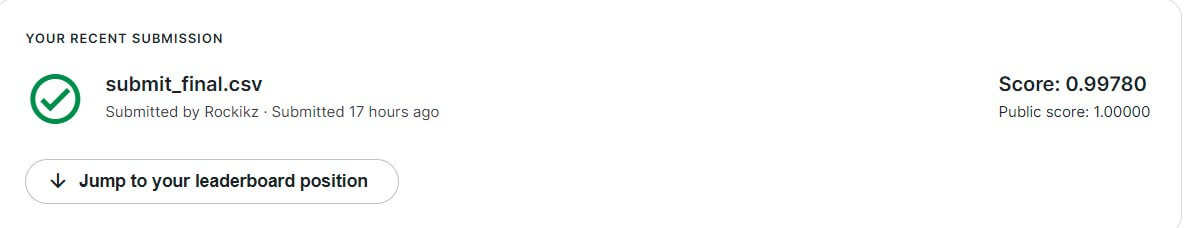
We got 99.78% and 100% accuracy on private and public leaderboards. That's awesome!
Conclusion
Alright, we're done with the tutorial. You can check this page to see various training parameters you can tweak.
If you have a custom fake news dataset for fine-tuning, you simply have to pass a list of samples to the tokenizer as we did, you won't change any other code after that.
Check the complete code here, or the Colab environment here.
Learn also: How to Perform Text Summarization using Transformers in Python
![]()
Happy learning ♥
Save time and energy with our Python Code Generator. Why start from scratch when you can generate? Give it a try!
View Full Code Explain The Code for Me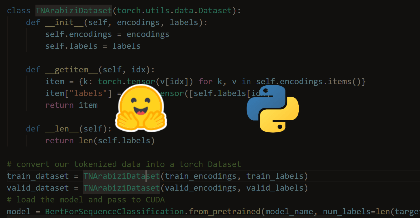


Got a coding query or need some guidance before you comment? Check out this Python Code Assistant for expert advice and handy tips. It's like having a coding tutor right in your fingertips!