Juggling between coding languages? Let our Code Converter help. Your one-stop solution for language conversion. Start now!
![]()
Introduction
Image captioning is the task of generating a text description of an input image. It involves both Computer Vision (such as Vision Transformers, or CNNs) and Natural Language Processing (NLP), such as language models.
Image captioning can help in many real-world applications, such as image search, providing a description of visual content to users with visual impairments, allowing them to better understand the content, and many more.
In this tutorial, you will learn how to perform image captioning using pre-trained models, as well as train your own model using PyTorch with the help of transformers library in Python.
Table of content:
- Introduction
- Model Architecture
- Image Captioning Datasets
- Getting Started
- Using a Trained Model
- Train your Own Image Captioning Model
- Models Evaluation
- Performing Inference
- Conclusion
Model Architecture
As you may already know, transformer architectures in neural networks have recently dominated the NLP field, with models like GPT and BERT has outperformed previous recurrent neural network architectures.
For computer vision, that's also the case now! When the paper "An Image is Worth 16x16 Words" was released, transformers also proved to be powerful in vision. Models like Vision Transformer (ViT), and DeiT have demonstrated state-of-the-art results in various computer vision tasks, such as image classification, object detection, image segmentation, and many more.
The below figure shows the ViT architecture, taken from the original paper:
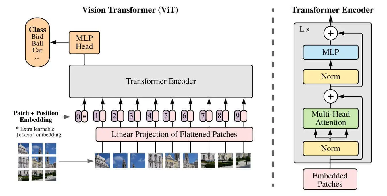
Figure 1: The Vision Transformer (ViT) architecture
The idea of Vision Transformer architecture is that it splits the image into fixed-size patches, these patches are flattened and then lower-dimensional linear embeddings are created from these patches. This way, it will behave as if it's a sequence of text.
Another Vision Transformer is the Swin Transformer, which adds the idea of Shifted Windows that brings greater efficiency by limiting self-attention computation to non-overlapping windows and still permitting cross-window connections. Here is the main difference between ViT and Swin, a figure taken from the Swin paper:
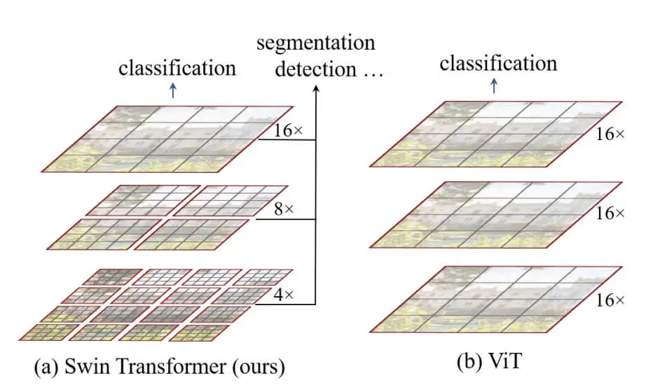
Figure 2: Swin Transformer vs ViT
Many research papers suggested that initializing image-to-text sequence models with pre-trained checkpoints has been shown to be effective, such as the TrOCR paper.
Therefore, in this tutorial, we will use Vision Encoder-Decoder architecture models, where the encoder is the ViT or Swin (or any other), and the decoder is a language model such as GPT2 or BERT, something like this:
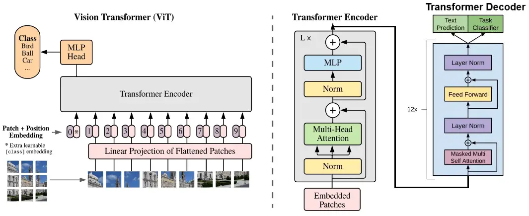
Figure 3: The Vision Encoder-Decoder architecture we'll use for image captioning
Image Captioning Datasets
The most common dataset for image captioning is the Common Objects in Context (COCO). We'll be using the 2014 version of it which contain more than 500,000 images and their descriptions.
There is the 2017 version of the COCO dataset, and also the Flickr30k which contains 31,000 images collected from Flickr. You're free to choose any dataset you want, or you can combine them if you know what you're doing.
Getting Started
In this tutorial, we will start by using models that are already trained so we can get a sense of how easy it is to get started with 🤗 Transformers.
Next, we'll train our own model using the COCO dataset using the Trainer class, and also using a regular PyTorch training loop, so you can pick the one that suits you best.
After that, we'll see how image captioning models are evaluated and which metrics are used to compare them.
Finally, we'll use our model to generate captions of any image we find on the Internet. Let's get started!
We will use the transformers library, as well as 🤗 evaluate and datasets libraries for proper model evaluation and downloading the dataset.
You can either use PyTorch or TensorFlow under transformers. I'll choose PyTorch for this:
$ pip install torch transformers rouge_score evaluate datasetsWe need the rouge_score library as it's a native implementation of the ROUGE score in Python, we'll see why it's needed in the next sections.
Of course, it's suggested that you use GPU for deep learning, as it'll be much faster, even during inference you'll notice a lot of improvements in terms of inference time. Head to this link to install PyTorch for your CUDA version. If you're on Google Colab, just ensure you're picking "GPU" in the notebook settings.
Open up a new Jupyter or Colab notebook, and import the following:
import requests
import torch
from PIL import Image
from transformers import *
from tqdm import tqdm
# set device to GPU if available
device = "cuda" if torch.cuda.is_available() else "cpu"
It's not suggested that you import everything from transformers as there will be a lot of classes and methods imported. Feel free to change it and only import what you need.
Throughout the tutorial, we'll be passing our model and data inputs to the device specified above. If CUDA is installed and available, then it'll be "cuda", and "cpu" otherwise.
Using a Trained Model
Next, let's download a fine-tuned image captioning model:
# load a fine-tuned image captioning model and corresponding tokenizer and image processor
finetuned_model = VisionEncoderDecoderModel.from_pretrained("nlpconnect/vit-gpt2-image-captioning").to(device)
finetuned_tokenizer = GPT2TokenizerFast.from_pretrained("nlpconnect/vit-gpt2-image-captioning")
finetuned_image_processor = ViTImageProcessor.from_pretrained("nlpconnect/vit-gpt2-image-captioning")
This model is a PyTorch version of the FLAX one that was fine-tuned on the COCO2017 dataset on a single epoch, you can see the training metrics here.
Let's try the model:
import urllib.parse as parse
import os

# a function to determine whether a string is a URL or not
def is_url(string):
    try:
        result = parse.urlparse(string)
        return all([result.scheme, result.netloc, result.path])
    except:
        return False

# a function to load an image
def load_image(image_path):
    if is_url(image_path):
        return Image.open(requests.get(image_path, stream=True).raw)
    elif os.path.exists(image_path):
        return Image.open(image_path)

# a function to perform inference
def get_caption(model, image_processor, tokenizer, image_path):
    image = load_image(image_path)
    # preprocess the image
    img = image_processor(image, return_tensors="pt").to(device)
    # generate the caption (using greedy decoding by default)
    output = model.generate(**img)
    # decode the output
    caption = tokenizer.batch_decode(output, skip_special_tokens=True)[0]
    return caption
The get_caption() function takes the model, the image processor, the tokenizer, and the image's path and performs inference on the model.
We simply call the model.generate() method and pass the outputs of the image processor, which are the pixel values of the image. Let's use it:
# load displayer
from IPython.display import display

url = "http://images.cocodataset.org/test-stuff2017/000000009384.jpg"
# display the image
display(load_image(url))
# get the caption
get_caption(finetuned_model, finetuned_image_processor, finetuned_tokenizer, url)
Output:
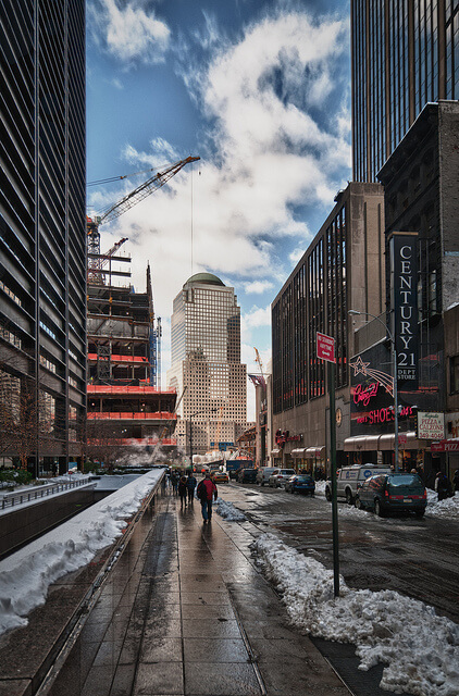
a person walking down a street with a snow covered sidewalk Excellent. You can pass any image you want, whether it's in your local environment or a URL just like we did here. You can check this XML file containing some test images on the COCO2017 dataset.
Train your Own Image Captioning Model
Loading the Model
Now that we're familiar with image captioning, let's fine-tune our model from pre-trained encoder and decoder models:
# the encoder model that process the image and return the image features
# encoder_model = "WinKawaks/vit-small-patch16-224"
# encoder_model = "google/vit-base-patch16-224"
# encoder_model = "google/vit-base-patch16-224-in21k"
encoder_model = "microsoft/swin-base-patch4-window7-224-in22k"
# the decoder model that process the image features and generate the caption text
# decoder_model = "bert-base-uncased"
# decoder_model = "prajjwal1/bert-tiny"
decoder_model = "gpt2"
# load the model
model = VisionEncoderDecoderModel.from_encoder_decoder_pretrained(
    encoder_model, decoder_model
).to(device)
As in demonstrated Figure 3, the encoder is a vision transformer that encodes the image into hidden vectors. The decoder is a regular language model that takes these hidden vectors and decodes them into human text.
For this demo, as mentioned earlier, we're going for Microsoft's Swin vision transformer that was pre-trained on ImageNet-21k (14 million images) at a resolution of 224x224. Check the Swin Transformer paper for more info regarding the details. As for the decoder, I'm choosing the gpt2 language model.
If you have limited computing resources, make sure you use smaller models such as the WinKawaks/vit-small-patch16-224 for the encoder and prajjwal1/bert-tiny for the decoder, you can uncomment them above.
To load the pre-trained weights of both models and combine them together in a single model, we use the VisionEncoderDecoderModel class and the from_encoder_decoder_pretrained() method that expects the name of both models. You can browse all the models in the huggingface hub.
Next, we have to load our image_processor and tokenizer:
# initialize the tokenizer
# tokenizer = AutoTokenizer.from_pretrained(decoder_model)
tokenizer = GPT2TokenizerFast.from_pretrained(decoder_model)
# tokenizer = BertTokenizerFast.from_pretrained(decoder_model)
# load the image processor
image_processor = ViTImageProcessor.from_pretrained(encoder_model)
We need the tokenizer to tokenize our captions into a sequence of integers using the GPT2TokenizerFast. If you're using a different decoder, make sure to comment this out and use the AutoTokenizer class. The reason I'm using it is that GPT2TokenizerFast is way faster than AutoTokenizer in case I'm using GPT2.
The ViTImageProcessor is responsible for processing our image before training/inferring, such as normalizing, resizing the image into the appropriate resolution, and scaling the pixel values.
Before proceeding, we have to make sure that the decoder_start_token_id and pad_token_id are present in our model configuration. Therefore, we have to manually set them using the tokenizer config:
if "gpt2" in decoder_model:
  # gpt2 does not have decoder_start_token_id and pad_token_id
  # but has bos_token_id and eos_token_id
  tokenizer.pad_token = tokenizer.eos_token # pad_token_id as eos_token_id
  model.config.eos_token_id = tokenizer.eos_token_id
  model.config.pad_token_id = tokenizer.pad_token_id
  # set decoder_start_token_id as bos_token_id
  model.config.decoder_start_token_id = tokenizer.bos_token_id
else:
  # set the decoder start token id to the CLS token id of the tokenizer
  model.config.decoder_start_token_id = tokenizer.cls_token_id
  # set the pad token id to the pad token id of the tokenizer
  model.config.pad_token_id = tokenizer.pad_token_id
Here is a definition of each special token defined above:
bos_token_idis the ID of the token that represents the beginning of the sentence.eos_token_idis the ID of the token that represents the end of the sentence.decoder_start_token_idis used to indicate the starting point of the decoder to start generating the target sequence (in our case, the caption).pad_token_idis used to pad short sequences of text into a fixed length.cls_token_idrepresents the classification token and is typically used by BERT and other tokenizers as the first token in a sequence of text before the actual sentence starts.
The GPT2 tokenizer does not have the pad_token_id and decoder_start_token_id but it has bos_token_id and eos_token_id. Therefore, we can simply set the pad_token as the eos_token and decoder_start_token_id as the bos_token_id.
For other language models such as BERT, we set the docoder_start_token_id as the cls_token_id.
The reason we're setting all of these is that when we assemble our model, these token ids are not loaded by default. If we do not set them now, we'll get weird errors later in training.
Downloading & Loading the Dataset
Now we've constructed our model, let's get into our dataset. As mentioned at the beginning, we will use the COCO2014 (Karpathy's annotations & splits):
from datasets import load_dataset

max_length = 32 # max length of the captions in tokens
coco_dataset_ratio = 50 # 50% of the COCO2014 dataset
train_ds = load_dataset("HuggingFaceM4/COCO", split=f"train[:{coco_dataset_ratio}%]")
valid_ds = load_dataset("HuggingFaceM4/COCO", split=f"validation[:{coco_dataset_ratio}%]")
test_ds = load_dataset("HuggingFaceM4/COCO", split="test")
len(train_ds), len(valid_ds), len(test_ds)
This will take more than 20 minutes of downloading if you're on Colab because it's more than 20GB in total size. COCO2017 is much bigger than that by the way.
Since we have limited computing resources, I'm only taking 50% of the total dataset. Nevertheless, here are the total samples of each set:
(283374, 12505, 25010)I'm taking the complete testing set so we can reliably compare models. Over 280K samples and that's only 50% of it. Feel free to change this ratio to a lower number if you just want to get going with the training, or to a higher one (possibly 100%) if you have a good GPU and time.
max_length is the maximum length of the caption, so our captions will only have 32 tokens as a maximum. If it's higher than that, the caption will be truncated. If it's lower than that, it'll be padded with the pad_token_id.
Next, during my initial training, I ran into some errors because some samples do not have 3 dimensions. Therefore, I'm filtering them out here:
import numpy as np

# remove the images with less than 3 dimensions (possibly grayscale images)
train_ds = train_ds.filter(lambda item: np.array(item["image"]).ndim in [3, 4], num_proc=2)
valid_ds = valid_ds.filter(lambda item: np.array(item["image"]).ndim in [3, 4], num_proc=2)
test_ds = test_ds.filter(lambda item: np.array(item["image"]).ndim in [3, 4], num_proc=2)
I'm using the .filter() method to only take images with the expected dimension. Setting num_proc to 2 will speed up the processing as it'll do it in two CPU cores. If you have more CPU cores, then increase this number to speed things up.
Preprocessing the Dataset
Now that we have valid samples, let's preprocess our inputs:
def preprocess(items):
  # preprocess the image
  pixel_values = image_processor(items["image"], return_tensors="pt").pixel_values.to(device)
  # tokenize the caption with truncation and padding
  targets = tokenizer([ sentence["raw"] for sentence in items["sentences"] ],
                      max_length=max_length, padding="max_length", truncation=True, return_tensors="pt").to(device)
  return {'pixel_values': pixel_values, 'labels': targets["input_ids"]}

# using with_transform to preprocess the dataset during training
train_dataset = train_ds.with_transform(preprocess)
valid_dataset = valid_ds.with_transform(preprocess)
test_dataset  = test_ds.with_transform(preprocess)
The preprocess() function expects the samples as parameters (items). We're preprocessing the image using our image processor, and tokenizing the captions with truncation and padding using our tokenizer. At the end of both, we pass them to the device using the to() method.
We could use the map() function to process our dataset. However, it may take too long and consume memory and storage in our case as it's a large dataset, and therefore we'll use the with_transform() so the preprocess() function will run only during training. In other words, the preprocessing happens on the fly when we pass the batches to the model.
Next, we define our function that collates the batches:
# a function we'll use to collate the batches
def collate_fn(batch):
    return {
        'pixel_values': torch.stack([x['pixel_values'] for x in batch]),
        'labels': torch.stack([x['labels'] for x in batch])
    }
We will pass the collate_fn() callback to our data loader before we start training.
Evaluation Metrics
There are a lot of metrics that emerged for image captioning, to mention a few:
- BLEU: It evaluates the n-gram overlap between the reference caption and the generated caption and gives a more balanced evaluation of content similarity and fluency. It is calculated by computing the precision of the generated text with respect to the reference text, and then taking the geometric average of the n-gram precisions (such as unigram, bigram, 3-gram, 4-gram, etc.). The most common version is BLEU-4, which considers the unigram to 4-gram overlap average. It is widely used in the machine translation task. Check this quick YouTube video to learn more about it, or you can check our tutorial about the BLEU score.
- ROUGE: It calculates the percentage of common tokens between the generated text and the reference text, with longer sequences given more weight. Like BLEU, the score is between 0 and 1, where 1 is the perfect match and 0 is the poorer match. ROUGE can be calculated using different n-gram orders, such as ROUGE-1 (unigrams, or just single token), ROUGE-2 (bigrams), or ROUGE-L (longest common subsequence). It is also common in machine translation and text summarization tasks. The most common version we'll use for image captioning is ROUGE-L. Check this YouTube video to learn more about it.
- METEOR: A combination of ROUGE and BLEU, which also considers word alignments, synonymy, and other factors.
- CIDEr: A metric that measures similarity between the generated text and reference texts using a consensus-based approach that takes into account the agreement among multiple human annotators.
- SPICE: A semantic-based metric that computes a graph-based representation of the captions and compares them based on their content. This metric is invented for image captioning specifically.
For this tutorial, we're going to stick with ROUGE-L and BLEU scores. The below code loads these metrics to compute them against a model:
import evaluate

# load the rouge and bleu metrics
rouge = evaluate.load("rouge")
bleu = evaluate.load("bleu")

def compute_metrics(eval_pred):
  preds = eval_pred.label_ids
  labels = eval_pred.predictions
  # decode the predictions and labels
  pred_str = tokenizer.batch_decode(preds, skip_special_tokens=True)
  labels_str = tokenizer.batch_decode(labels, skip_special_tokens=True)
  # compute the rouge score
  rouge_result = rouge.compute(predictions=pred_str, references=labels_str)
  # multiply by 100 to get the same scale as the rouge score
  rouge_result = {k: round(v * 100, 4) for k, v in rouge_result.items()}
  # compute the bleu score
  bleu_result = bleu.compute(predictions=pred_str, references=labels_str)
  # get the length of the generated captions
  generation_length = bleu_result["translation_length"]
  return {
        **rouge_result,
        "bleu": round(bleu_result["bleu"] * 100, 4),
        "gen_len": bleu_result["translation_length"] / len(preds)
  }
The compute_metrics() function takes the EvalPrediction object to compute the ROUGE and BLEU scores after decoding them using the tokenizer, we also multiply the scores by 100.
Let's define some basic training parameters:
num_epochs = 2 # number of epochs
batch_size = 16 # the size of batches
We're going through the dataset twice. Again, if you have more computing, make sure to increase the num_epochs to say 10. At the time of writing this, the free version of the Colab instance gives us NVIDIA Tesla T4 which fits a batch_size of 16 very well and does not raise any Out of Memory errors.
If you have a GPU with more VRAM, you should increase the batch_size to take the most advantage of your GPU and speed up the training.
Before we proceed with training, let's print a single sample to see whether the shapes are as expected:
for item in train_dataset:
  print(item["labels"].shape)
  print(item["pixel_values"].shape)
  break
I'm iterating over the training dataset and printing the shapes of labels and pixel_values. Here's the output:
torch.Size([32])
torch.Size([3, 224, 224])
PyTorch tensors with the expected shape, labels is the caption with the size of max_length=32, and the pixel_values is the actual image with (3, 224, 224) resolution.
Training
For training, we have two choices. The first one is using the Trainer class that is provided by the transformers library, which is convenient and very simple to use. Or you can use the regular PyTorch training loop if you want. I will show you how to do both, and you're free to show any of them.
Using the Trainer Class
Let's define the training arguments:
# define the training arguments
training_args = Seq2SeqTrainingArguments(
    predict_with_generate=True,             # use generate to calculate the loss
    num_train_epochs=num_epochs,            # number of epochs
    evaluation_strategy="steps",            # evaluate after each eval_steps
    eval_steps=2000,                        # evaluate after each 2000 steps
    logging_steps=2000,                     # log after each 2000 steps
    save_steps=2000,                        # save after each 2000 steps
    per_device_train_batch_size=batch_size, # batch size for training
    per_device_eval_batch_size=batch_size,  # batch size for evaluation
    output_dir="vit-swin-base-224-gpt2-image-captioning", # output directory
    # push_to_hub=True # whether you want to push the model to the hub,
    # check this guide for more details: https://huggingface.co/transformers/model_sharing.html
)
We will evaluate, log, and save the model checkpoint every 2000 steps, you're always encouraged to change this value depending on your batch_size, num_epochs and coco_dataset_ratio.
There are about 100 parameters you can pass to Seq2SeqTrainingArguments, check the doc reference if you're curious.
Next, we pass the training arguments to our actual trainer, along with the collation and compute_metrics() functions, model, and all the datasets:
# instantiate trainer
trainer = Seq2SeqTrainer(
    model=model,                     # the instantiated 🤗 Transformers model to be trained
    tokenizer=image_processor,       # we use the image processor as the tokenizer
    args=training_args,              # pass the training arguments
    compute_metrics=compute_metrics,
    train_dataset=train_dataset,
    eval_dataset=valid_dataset,
    data_collator=collate_fn,
)
The documentation encourages us to subclass the Trainer to define our own trainer so we can do custom behaviors with certain classes. Since I'm too lazy for that, I'm just overriding get_training_dataloder(), get_eval_dataloader(), and get_test_dataloader() functions to return a regular PyTorch DataLoader:
from torch.utils.data import DataLoader

def get_eval_loader(eval_dataset=None):
  return DataLoader(valid_dataset, collate_fn=collate_fn, batch_size=batch_size)

def get_test_loader(eval_dataset=None):
  return DataLoader(test_dataset, collate_fn=collate_fn, batch_size=batch_size)

# override the get_train_dataloader, get_eval_dataloader and
# get_test_dataloader methods of the trainer
# so that we can properly load the data
trainer.get_train_dataloader = lambda: DataLoader(train_dataset, collate_fn=collate_fn, batch_size=batch_size)
trainer.get_eval_dataloader = get_eval_loader
trainer.get_test_dataloader = get_test_loader
Let's fine-tune the model now:
# train the model
trainer.train()
This will take several hours to train, here's an output during my training of Abdou/vit-swin-base-224-gpt2-image-captioning:
 [10602/10602 5:08:53, Epoch 2/2]
Step	Training Loss	Validation Loss	Rouge1	    Rouge2	Rougel	Rougelsum	Bleu	    Gen Len
2000	1.0018	        0.8859	        38.6537	    13.8145	35.3932	35.393500	8.244800	11.294636
4000	0.8827	        0.8394	        40.0458	    14.8829	36.5321	36.536600	9.116900	11.294636
6000	0.8378	        0.8139	        41.2736	    15.9576	37.5504	37.551200	9.871000	11.294636
8000	0.7913	        0.8011	        41.6642	    16.1987	37.8786	37.889100	10.078600	11.294636
10000	0.7794	        0.7933	        41.9119	    16.3738	38.1062	38.129200	10.288000	11.294636
TrainOutput(global_step=10602, training_loss=0.8540051526291104, metrics={'train_runtime': 18543.3546, 'train_samples_per_second': 36.59, 'train_steps_per_second': 0.572, 'total_flos': 1.2314333621526567e+20, 'train_loss': 0.8540051526291104, 'epoch': 2.0})
The above output was using batch_size of 64. The training ended in approximately 5 hours on NVIDIA A100 GPU. You can further increase the coco_dataset_ratio and num_epochs to increase the scores.
These scores (ROUGE-1, ROUGE-2, ROUGE-L, BLEU) are calculated on the validation set. Let's evaluate our model on the test set:
# evaluate on the test_dataset
trainer.evaluate(test_dataset)
Output:
{'eval_loss': 0.7923195362091064,
 'eval_rouge1': 41.8451,
 'eval_rouge2': 16.3493,
 'eval_rougeL': 38.0288,
 'eval_rougeLsum': 38.049,
 'eval_bleu': 10.2776,
 'eval_gen_len': 11.294636296840558,
 'eval_runtime': 386.5944,
 'eval_samples_per_second': 38.725,
 'eval_steps_per_second': 0.605,
 'epoch': 2.0}
Amazing, we got a BLEU score of ~10.28, and a ROUGE-L of ~38.03 with the predict_with_generate parameter set to True.
Using PyTorch Training Loop
For the people who like flexibility in training, I have made this available to you. Let's wrap our training, validation, and testing sets as data loaders:
# alternative way of training: pytorch loop
from torch.utils.data import DataLoader

# define our data loaders
train_dataset_loader = DataLoader(train_dataset, collate_fn=collate_fn, batch_size=batch_size, shuffle=True)
valid_dataset_loader = DataLoader(valid_dataset, collate_fn=collate_fn, batch_size=8, shuffle=True)
test_dataset_loader = DataLoader(test_dataset, collate_fn=collate_fn, batch_size=8, shuffle=True)
Defining the optimizer:
from torch.optim import AdamW

# define the optimizer
optimizer = AdamW(model.parameters(), lr=1e-5)
I'm choosing AdamW optimizer as in the Trainer API. A learning rate of 1e-5 is no way near the optimal, feel free to play around with it.
Optionally, loading tensorboard on notebooks:
# start tensorboard
%load_ext tensorboard
%tensorboard --logdir ./image-captioning/tensorboard
Next, defining some variables and the summary tensorboard writer:
from torch.utils.tensorboard import SummaryWriter

summary_writer = SummaryWriter(log_dir="./image-captioning/tensorboard")
# print some statistics before training
# number of training steps
n_train_steps = num_epochs * len(train_dataset_loader)
# number of validation steps
n_valid_steps = len(valid_dataset_loader)
# current training step
current_step = 0
# logging, eval & save steps
save_steps = 1000
Here's the training loop now:
for epoch in range(num_epochs):
    # set the model to training mode
    model.train()
    # initialize the training loss
    train_loss = 0
    for batch in tqdm(train_dataset_loader, "Training", total=len(train_dataset_loader), leave=False):
      if current_step % save_steps == 0:
        ### evaluation code ###
        # evaluate on the validation set
        # if the current step is a multiple of the save steps
        print(f"\nValidation at step {current_step}...\n")
        # set the model to evaluation mode
        model.eval()
        # initialize our lists that store the predictions and the labels
        predictions, labels = [], []
        # initialize the validation loss
        valid_loss = 0
        for batch in valid_dataset_loader:
            # get the batch
            pixel_values = batch["pixel_values"]
            label_ids = batch["labels"]
            # forward pass
            outputs = model(pixel_values=pixel_values, labels=label_ids)
            # get the loss
            loss = outputs.loss
            valid_loss += loss.item()
            # free the GPU memory
            logits = outputs.logits.detach().cpu()
            # add the predictions to the list
            predictions.extend(logits.argmax(dim=-1).tolist())
            # add the labels to the list
            labels.extend(label_ids.tolist())
        # make the EvalPrediction object that the compute_metrics function expects
        eval_prediction = EvalPrediction(predictions=predictions, label_ids=labels)
        # compute the metrics
        metrics = compute_metrics(eval_prediction)
        # print the stats
        print(f"\nEpoch: {epoch}, Step: {current_step}, Train Loss: {train_loss / save_steps:.4f}, " +
              f"Valid Loss: {valid_loss / n_valid_steps:.4f}, BLEU: {metrics['bleu']:.4f}, " +
              f"ROUGE-1: {metrics['rouge1']:.4f}, ROUGE-2: {metrics['rouge2']:.4f}, ROUGE-L: {metrics['rougeL']:.4f}\n")
        # log the metrics
        summary_writer.add_scalar("valid_loss", valid_loss / n_valid_steps, global_step=current_step)
        summary_writer.add_scalar("bleu", metrics["bleu"], global_step=current_step)
        summary_writer.add_scalar("rouge1", metrics["rouge1"], global_step=current_step)
        summary_writer.add_scalar("rouge2", metrics["rouge2"], global_step=current_step)
        summary_writer.add_scalar("rougeL", metrics["rougeL"], global_step=current_step)
        # save the model
        model.save_pretrained(f"./image-captioning/checkpoint-{current_step}")
        tokenizer.save_pretrained(f"./image-captioning/checkpoint-{current_step}")
        image_processor.save_pretrained(f"./image-captioning/checkpoint-{current_step}")
        # get the model back to train mode
        model.train()
        # reset the train and valid loss
        train_loss, valid_loss = 0, 0
      ### training code below ###
      # get the batch & convert to tensor
      pixel_values = batch["pixel_values"]
      labels = batch["labels"]
      # forward pass
      outputs = model(pixel_values=pixel_values, labels=labels)
      # get the loss
      loss = outputs.loss
      # backward pass
      loss.backward()
      # update the weights
      optimizer.step()
      # zero the gradients
      optimizer.zero_grad()
      # log the loss
      loss_v = loss.item()
      train_loss += loss_v
      # increment the step
      current_step += 1
      # log the training loss
      summary_writer.add_scalar("train_loss", loss_v, global_step=current_step)
In the training loop, we're doing the forward and backward pass, updating the weights using the optimizer.step() and zeroing the gradients.
If the current_step is a multiple of the save_steps, then we perform the evaluation on the validation set, print out the metrics and add them to the tensorboard. I ran the training and here's how the output looks like:
Training:   0%|          | 0/17669 [00:00<?, ?it/s]
Validation at step 1000...

Epoch: 0, Step: 1000, Train Loss: 0.0000, Valid Loss: 1.0927, BLEU: 8.1102, ROUGE-1: 42.6778, ROUGE-2: 13.0396, ROUGE-L: 40.6797

Training:   6%|▌         | 1000/17669 [24:51<4:38:49,  1.00s/it]
Validation at step 2000...

Epoch: 0, Step: 2000, Train Loss: 1.0966, Valid Loss: 0.9991, BLEU: 10.8885, ROUGE-1: 46.1669, ROUGE-2: 16.6826, ROUGE-L: 44.4348

Training:  11%|█▏        | 2000/17669 [49:38<4:33:30,  1.05s/it]
Validation at step 3000...

Epoch: 0, Step: 3000, Train Loss: 1.0323, Valid Loss: 0.9679, BLEU: 11.6235, ROUGE-1: 47.1454, ROUGE-2: 17.6634, ROUGE-L: 45.5163

Model weights saved in ./image-captioning/checkpoint-3000/pytorch_model.bin
I stopped the training after 3000 steps, so it's working!
I see that the metrics are best after 3000 steps (I'm sure you can get better results if you continue training). Let's load that model:
# load the best model, change the checkpoint number to the best checkpoint
# if the last checkpoint is the best, then ignore this cell
best_checkpoint = 3000
best_model = VisionEncoderDecoderModel.from_pretrained(f"./image-captioning/checkpoint-{best_checkpoint}").to(device)
Models Evaluation
In this section, we are going to evaluate three different models:
- The one we just trained using the PyTorch training loop.
- The already fine-tuned
nlpconnect/vit-gpt2-image-captioning. - The model I fine-tuned using the
Trainerclass and is pushed to the hub,Abdou/vit-swin-base-224-gpt2-image-captioning.
First, let's make the function that takes the model and dataset as input, and return the metrics for that model:
def get_evaluation_metrics(model, dataset):
  model.eval()
  # define our dataloader
  dataloader = DataLoader(dataset, collate_fn=collate_fn, batch_size=batch_size)
  # number of testing steps
  n_test_steps = len(dataloader)
  # initialize our lists that store the predictions and the labels
  predictions, labels = [], []
  # initialize the test loss
  test_loss = 0.0
  for batch in tqdm(dataloader, "Evaluating"):
      # get the batch
      pixel_values = batch["pixel_values"]
      label_ids = batch["labels"]
      # forward pass
      outputs = model(pixel_values=pixel_values, labels=label_ids)
      # outputs = model.generate(pixel_values=pixel_values, max_length=max_length)
      # get the loss
      loss = outputs.loss
      test_loss += loss.item()
      # free the GPU memory
      logits = outputs.logits.detach().cpu()
      # add the predictions to the list
      predictions.extend(logits.argmax(dim=-1).tolist())
      # add the labels to the list
      labels.extend(label_ids.tolist())
  # make the EvalPrediction object that the compute_metrics function expects
  eval_prediction = EvalPrediction(predictions=predictions, label_ids=labels)
  # compute the metrics
  metrics = compute_metrics(eval_prediction)
  # add the test_loss to the metrics
  metrics["test_loss"] = test_loss / n_test_steps
  return metrics
It's quite similar (maybe even identical) to the evaluation code in the training loop we wrote earlier. Let's use this function to evaluate our best_model we just trained:
metrics = get_evaluation_metrics(best_model, test_dataset)
metrics
Evaluating: 100%|██████████| 6230/6230 [17:10<00:00, 6.04it/s]
{'rouge1': 46.9427,
'rouge2': 17.659,
'rougeL': 45.2971,
'rougeLsum': 45.2916,
'bleu': 11.7049,
'gen_len': 11.262560192616373,
'test_loss': 0.9731424459819809}Next, remember we loaded the nlpconnect/vit-gpt2-image-captioning model at the beginning of this tutorial, let's evaluate it on the COCO2014 testing set:
get_evaluation_metrics(finetuned_model, test_dataset)
{'rouge1': 48.624,
 'rouge2': 20.5349,
 'rougeL': 47.0933,
 'rougeLsum': 47.0975,
 'bleu': 11.7336,
 'gen_len': 11.262560192616373,
 'test_loss': 9.437558887552106}
This is slightly better on almost all the metrics, the reason is that this one is fine-tuned on a whole epoch (and not only 3000 steps) on the COCO2017 dataset.
Let's now load the Abdou/vit-swin-base-224-gpt2-image-captioning model using the simple pipeline API and do the evaluation:
# using the pipeline API
image_captioner = pipeline("image-to-text", model="Abdou/vit-swin-base-224-gpt2-image-captioning")
image_captioner.model = image_captioner.model.to(device)
get_evaluation_metrics(image_captioner.model, test_dataset){'rouge1': 53.1153,
'rouge2': 24.2307,
'rougeL': 51.5002,
'rougeLsum': 51.4983,
'bleu': 17.7765,
'gen_len': 11.262560192616373,
'test_loss': 0.7988893618313879}That's much better than the previous two. In the next section, we'll have fun with these models and predict some images.
Performing Inference
In the end, let's predict the captions of some sample images grabbed from the COCO2017 testing set:
def show_image_and_captions(url):
  # get the image and display it
  display(load_image(url))
  # get the captions on various models
  our_caption = get_caption(best_model, image_processor, tokenizer, url)
  finetuned_caption = get_caption(finetuned_model, finetuned_image_processor, finetuned_tokenizer, url)
  pipeline_caption = get_caption(image_captioner.model, image_processor, tokenizer, url)
  # print the captions
  print(f"Our caption: {our_caption}")
  print(f"nlpconnect/vit-gpt2-image-captioning caption: {finetuned_caption}")
  print(f"Abdou/vit-swin-base-224-gpt2-image-captioning caption: {pipeline_caption}")
Below are some examples:
show_image_and_captions("http://images.cocodataset.org/test-stuff2017/000000000001.jpg")Output:
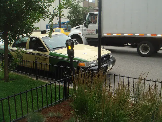
Our caption: A truck parked in a parking lot with a man on the back.
nlpconnect/vit-gpt2-image-captioning caption: a green truck parked next to a curb
Abdou/vit-swin-base-224-gpt2-image-captioning caption: A police car parked next to a fence.
A second example:
show_image_and_captions("http://images.cocodataset.org/test-stuff2017/000000000019.jpg")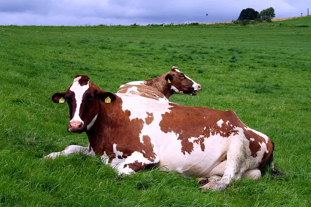
Our caption: A cow standing in a field with a bunch of grass.
nlpconnect/vit-gpt2-image-captioning caption: a cow is standing in a field of grass
Abdou/vit-swin-base-224-gpt2-image-captioning caption: Two cows laying in a field with a sky background.
The first two models didn't see the second cow in the back! Here's a third example:
show_image_and_captions("http://images.cocodataset.org/test-stuff2017/000000000128.jpg")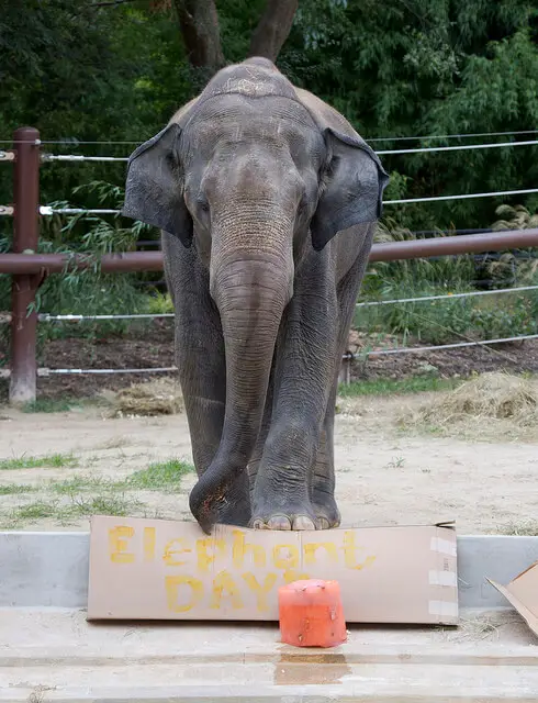
Our caption: A large elephant standing in a dirt field.
nlpconnect/vit-gpt2-image-captioning caption: an elephant with a large trunk standing on a dirt ground
Abdou/vit-swin-base-224-gpt2-image-captioning caption: An elephant standing next to a box on a cement ground.
Here's a final example:
show_image_and_captions("http://images.cocodataset.org/test-stuff2017/000000003720.jpg")
Our caption: A woman standing on a sidewalk with a umbrella.
nlpconnect/vit-gpt2-image-captioning caption: a person walking down a street holding an umbrella
Abdou/vit-swin-base-224-gpt2-image-captioning caption: A woman holding an umbrella walking down a sidewalk.
Conclusion
Alright! We have covered a lot in this article:
- First, we saw how to load a fine-tuned model and perform inference on it.
- Then, we learned how to fine-tune our own model using either
transformers'TrainerAPI or PyTorch. - Finally, we compared the results of three models on various test inputs.
Here are some of the suggestions to further improve the results:
- I invite you to explore
Salesforce/blip-image-captioning-basemodel, it can be used both as conditional or unconditional image captioning. - If you have more computing resources, then increase the number of epochs and set
coco_dataset_ratioto 100, and set it to training for more hours. In case you obtain improved results, feel free to share your weights on the HuggingFace hub. This link should help you. - You can also experiment with other vision transformers, such as the regular ViT, or BEiT.
- Additionally, you can try out different language models like BERT, RoBERTa, and others.
- Add the METEOR metric to the
compute_metrics()method, this link will help.
Related articles:
- How to Fine Tune BERT for Text Classification using Transformers in Python
- Conversational AI Chatbot with Transformers in Python
- Skin Cancer Detection using TensorFlow in Python
References and useful links:
- Vision Encoder-Decoder Models - Transformers
- Swin Transformer - Huggingface
nlpconnect/vit-gpt2-image-captioning- Image Captioning Datasets - Papers With Code
You can get the complete code here. Alternatively, follow this link for the Colab version.
![]()
Happy learning ♥
Ready for more? Dive deeper into coding with our AI-powered Code Explainer. Don't miss it!
View Full Code Explain My Code


Got a coding query or need some guidance before you comment? Check out this Python Code Assistant for expert advice and handy tips. It's like having a coding tutor right in your fingertips!