How to Perform Malaria Classification using TensorFlow 2 and Keras in Python

Sofiane Ouaari · 9 min read · Updated may 2022 · Machine Learning · Computer Vision · Healthcare

Ready to take Python coding to a new level? Explore our Python Code Generator. The perfect tool to get your code up and running in no time. Start now!

Disclosure: This post may contain affiliate links, meaning when you click the links and make a purchase, we receive a commission.

Deep Learning use cases in medicine have known a big leap those past years, from patient automatic diagnosis to computer vision, many cutting-edge models are being developed in this domain.

In this tutorial, we will implement a deep learning model using TensorFlow (Keras API) for a binary classification task which consists of labeling cells' images into either infected or not with Malaria.

Installing required libraries and frameworks:

pip install numpy tensorflow opencv-python sklearn matplotlib

Downloading the Dataset

We gonna be using Malaria Cell Images Dataset from Kaggle, after downloading and unzipping the folder, you'll see cell_images, this folder will contain two subfolders: Parasitized, Uninfected and another duplicated cell_images folder, feel free to delete that one.

I also invite you to move an image from both classes to another folder testing-samples, so we can make inferences on it when we finish training our model.

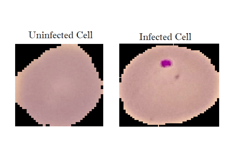Image Preprocessing with OpenCV

OpenCV is an optimized open-source library for image processing and computer vision. We will use it to preprocess our images and turn them to greyscale in the form of a NumPy array (numerical format) and resize it to a (70x70) shape:

import cv2
import tensorflow as tf
from tensorflow.keras.models import Sequential 
from tensorflow.keras.layers import Dense, Conv2D, MaxPool2D, Flatten, Activation
from sklearn.model_selection import train_test_split
import numpy as np
import matplotlib.pyplot as plt
import glob
import os

# after you extract the dataset, 
# put cell_images folder in the working directory
img_dir="cell_images"  
img_size=70

def load_img_data(path):
    image_files = glob.glob(os.path.join(path, "Parasitized/*.png")) + \
                  glob.glob(os.path.join(path, "Uninfected/*.png"))
    X, y = [], []
    for image_file in image_files:
        # 0 for uninfected and 1 for infected
        label = 0 if "Uninfected" in image_file else 1
        # load the image in gray scale
        img_arr = cv2.imread(image_file, cv2.IMREAD_GRAYSCALE)
        # resize the image to (70x70)
        img_resized = cv2.resize(img_arr, (img_size, img_size))
        X.append(img_resized)
        y.append(label)
    return X, y

We used glob built-in module to get all images in that format (ending with .png in a specific folder).

Then we iterate over these image file names and load each image in grayscale, resize it and append it to our array, we also do the same for labels (0 for uninfected and 1 for parasitized).

Preparing and Normalizing the Dataset

Now that we have our function to load the dataset, let's call it and perform some preparation:

# load the data
X, y = load_img_data(img_dir)
# reshape to (n_samples, 70, 70, 1) (to fit the NN)
X = np.array(X).reshape(-1, img_size, img_size, 1)
# scale pixels from the range [0, 255] to [0, 1] 
# to help the neural network learn much faster
X = X / 255 

# shuffle & split the dataset
X_train, X_test, y_train, y_test = train_test_split(X, y, test_size=0.1, stratify=y)
print("Total training samples:", X_train.shape)
print("Total validation samples:", X_test.shape[0])

After we load our dataset preprocessed, we extend our images array shape into (n_samples, 70, 70, 1) to fit the neural network input.

In addition, to help the network converge faster, we should perform data normalization. There are scaling methods from that in sklearn such as:

StandardScaler: x_norm = (x - mean) / std (where std is the Standard Deviation)
MinMaxScaler: x_norm = (x - x_min) / (x_max - x_min) this results to x_norm ranging between 0 and 1.

In our case, we won't be using those. Instead, we will divide by 255 since the biggest value a pixel can achieve is 255, this will results to pixels ranging between 0 and 1 after applying the scaling.

Then we will use the train_test_split() method from sklearn to divide the dataset into training and testing sets, we used 10% of the total data for validation it later on. The stratify parameter will preserve the proportion of target as in the original dataset, in the train and test datasets as well.

train_test_split() method shuffles the data by default (shuffle is set to True), we want to do that, since the original ordering is composed of straight 0s labels in the first half and straight 1s labels in the second half, which may result in bad training of the network later on.

Implementing the CNN Model Architecture

Our neural network architecture will follow somehow the same architecture presented in the figure:

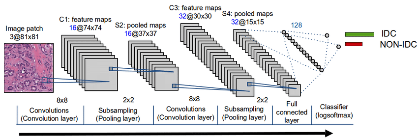
In our case, we will add 3 convolution layers then we Flatten to be followed by fully connected layers composed by Dense layers.

Let us define those layers and properties:

Convolution Layers: The role of convolution layers is to reduce the images into easier forms by maintaining only the most important features. A matrix filter will traverse the images to apply the convolution operations.
Pooling Layers: Their role consists in reducing the spacial volume resulted from the convolution operations. There are two types of pooling layers; average pooling layers and max-pooling layers (in our case we will use the latter).
Flatten: A layer responsible for transforming the results from the convolution and polling into a 1D shape to be feed-forwarded afterward in a fully connected layer.

model = Sequential()
model.add(Conv2D(64, (3, 3), input_shape=X_train.shape[1:]))
model.add(Activation("relu"))
model.add(MaxPool2D(pool_size=(2, 2)))

model.add(Conv2D(64, (3, 3)))
model.add(Activation("relu"))
model.add(MaxPool2D(pool_size=(2, 2)))

model.add(Conv2D(64, (3, 3)))
model.add(Activation("relu"))
model.add(MaxPool2D(pool_size=(2, 2)))

model.add(Flatten())

model.add(Dense(64))
model.add(Activation("relu"))

model.add(Dense(64))
model.add(Activation("relu"))

model.add(Dense(1))
model.add(Activation("sigmoid"))

model.compile(loss="binary_crossentropy", optimizer="adam", metrics=["accuracy"])

# train the model with 3 epochs, 64 batch size
model.fit(X_train, np.array(y_train), batch_size=64, epochs=3, validation_split=0.2)
# if you already trained the model, uncomment below and comment above
# so you can only load the previously trained model
# model.load_weights("malaria-cell-cnn.h5")

Since the output is binary (either infected or not infected) we have used Sigmoid (1/(1+exp(-x)) as the activation function of the output layer.

Here is my training output:

Train on 19840 samples, validate on 4960 samples
Epoch 1/3
19840/19840 [==============================] - 14s 704us/sample - loss: 0.5067 - accuracy: 0.7135 - val_loss: 0.1949 - val_accuracy: 0.9300
Epoch 2/3
19840/19840 [==============================] - 12s 590us/sample - loss: 0.1674 - accuracy: 0.9391 - val_loss: 0.1372 - val_accuracy: 0.9482
Epoch 3/3
19840/19840 [==============================] - 12s 592us/sample - loss: 0.1428 - accuracy: 0.9495 - val_loss: 0.1344 - val_accuracy: 0.9518

As you may have noticed, we achieved an accuracy of 95% on the training dataset and its validation split.

Model Evaluation

Now let us use the evaluate() from Keras API to evaluate the model on the testing dataset:

loss, accuracy = model.evaluate(X_test, np.array(y_test), verbose=0)
print(f"Testing on {len(X_test)} images, the results are\n Accuracy: {accuracy} | Loss: {loss}")

Testing on 2756 images, the results are
 Accuracy: 0.9444847702980042 | Loss: 0.15253388267470028

The model performed well also in the test data with an accuracy reaching 94%.

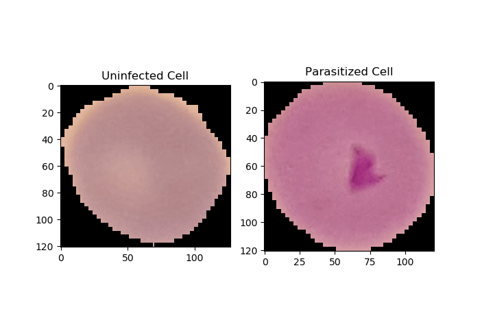
Now let's use this model to make inferences on the two images we put in the testing-samples folder earlier in this tutorial. First, let's plot them:

# testing some images
uninfected_cell = "cell_images/testing-samples/C1_thinF_IMG_20150604_104919_cell_82.png"
infected_cell = "cell_images/testing-samples/C38P3thinF_original_IMG_20150621_112116_cell_204.png"

_, ax = plt.subplots(1, 2)
ax[0].imshow(plt.imread(uninfected_cell))
ax[0].title.set_text("Uninfected Cell")
ax[1].imshow(plt.imread(infected_cell))
ax[1].title.set_text("Parasitized Cell")
plt.show()

Output:

Malaria Infected vs Uninfected Cells

Great, now let's load these images and perform preprocessing:

img_arr_uninfected = cv2.imread(uninfected_cell, cv2.IMREAD_GRAYSCALE)
img_arr_infected = cv2.imread(infected_cell, cv2.IMREAD_GRAYSCALE)
# resize the images to (70x70)
img_arr_uninfected = cv2.resize(img_arr_uninfected, (img_size, img_size))
img_arr_infected = cv2.resize(img_arr_infected, (img_size, img_size))
# scale to [0, 1]
img_arr_infected = img_arr_infected / 255
img_arr_uninfected = img_arr_uninfected / 255
# reshape to fit the neural network dimensions
# (changing shape from (70, 70) to (1, 70, 70, 1))
img_arr_infected = img_arr_infected.reshape(1, *img_arr_infected.shape)
img_arr_infected = np.expand_dims(img_arr_infected, axis=3)
img_arr_uninfected = img_arr_uninfected.reshape(1, *img_arr_uninfected.shape)
img_arr_uninfected = np.expand_dims(img_arr_uninfected, axis=3)

All we have to do now is to use predict() method to make inference:

# perform inference
infected_result = model.predict(img_arr_infected)[0][0]
uninfected_result = model.predict(img_arr_uninfected)[0][0]
print(f"Infected: {infected_result}")
print(f"Uninfected: {uninfected_result}")

Output:

Infected: 0.9827326536178589
Uninfected: 0.005085020791739225

Awesome, the model is 98% sure that the infected cell is in fact infected, and he's sure 99.5% of the time that the uninfected cell is uninfected.

Saving the model

Finally, we will conclude all this process by saving our model.

# save the model & weights
model.save("malaria-cell-cnn.h5")

Conclusion:

In this tutorial you have learned:

How to process raw images, convert them in greyscale and in a NumPy array (numerical format) using OpenCV.
The architecture behind a Convolutional Neural Network with its various components.
To implement a CNN in a Tensorflow/Keras.
To evaluate, and save a deep learning model, as well as performing inference on it.

I encourage you to tweak the model parameters, or you may want to use transfer learning so you can perform much better. You can also train on colored images instead of greyscale, this may help!

There are other metrics besides accuracy, such as sensitivity and specificity, which are widely used in the medical field, I invite you to add them here as well. If you're not sure how there is a tutorial on skin cancer detection in which we did all of that!

Want to Learn More?

Finally, I've collected some useful resources and courses for you for further learning, here you go:

Learn also: Skin Cancer Detection using TensorFlow in Python.

Happy Learning ♥

Want to code smarter? Our Python Code Assistant is waiting to help you. Try it now!

View Full Code Understand My Code

Sharing is caring!

Read Also

Skin Cancer Detection using TensorFlow in Python

Comment panel

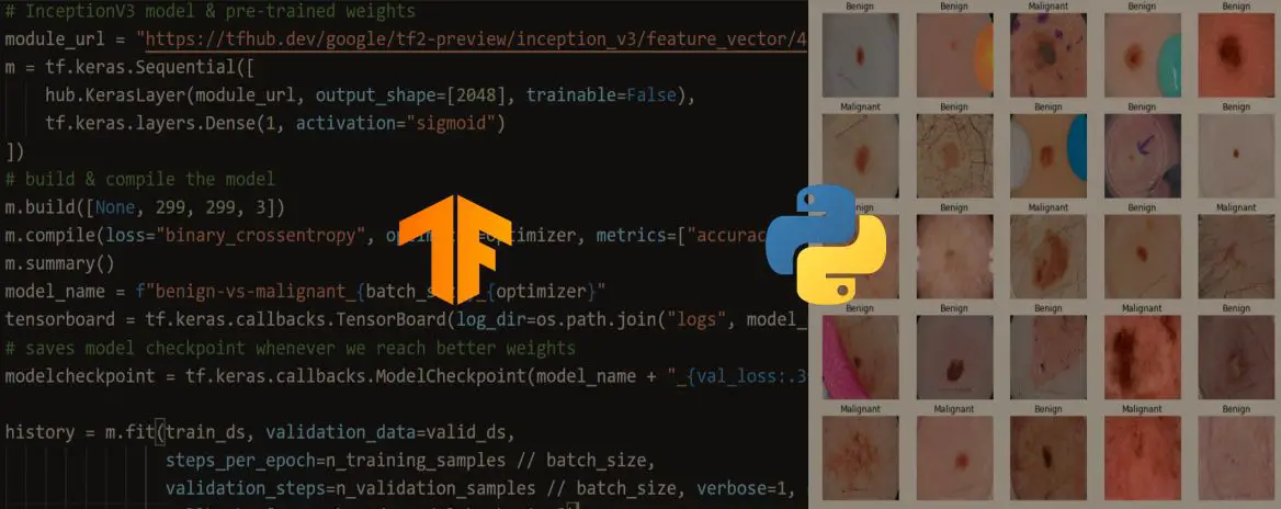
Got a coding query or need some guidance before you comment? Check out this Python Code Assistant for expert advice and handy tips. It's like having a coding tutor right in your fingertips!