Clustering Algorithms in Machine Learning with Python

  Mohtashim Nawaz · 33 min read · Updated jan 2023 · Machine Learning

Get a head start on your coding projects with our Python Code Generator. Perfect for those times when you need a quick solution. Don't wait, try it today!

Introduction

Data is the heart of machine learning algorithms. It defines how an algorithm would work, what it will output, and how it will be useful in the real world. Speaking in terms of labeling, you can have three types of data as given below.

• Labeled data: As the name suggests, you would have all the data samples labeled with a specific class. It is difficult to find labeled data in real life, and often expensive.
• Unlabeled data: In this category, none of the data samples are labeled.
• Semi-labeled data: When some of the data points are labeled and some are unlabeled, it is called semi-labeled data.

In the real world, you would find unlabeled data very often. It is because data labeling needs expertise and time, both of which are costly. 

Therefore, the experts have developed methods to work with unlabeled and semi-labeled data. Clustering is one such technique. It aims at finding the hidden patterns in the data without needing any labels. 

This article explores clustering algorithms in machine learning including the classic clustering algorithms and newly developed methods, example codes of each algorithm, and their results on sample datasets. But let us first understand what is clustering and how it works.

Table of Contents

• Clustering and its Need in Machine Learning
• Types of Clustering
  • Density-based Clustering
  • Distribution-based Clustering
  • Centroid-based Clustering
  • Hierarchical Clustering
• Other Classifications of Clustering Algorithms
  • Hard Clustering and Soft Clustering
  • Monothetic Clustering and Polythetic Clustering
• Popular Clustering Algorithms
  • Library Installation
  • K-means Clustering
  • Mini Batch K-means Clustering
  • Affinity Propagation
  • DBSCAN Clustering Algorithm
  • OPTICS
  • BIRCH
  • Agglomerative Clustering
  • Mean-Shift Clustering
  • Spectral Clustering
  • Gaussian Mixture Model
• Metrics for Evaluation of Clustering Algorithms
  • Homogeneity Score
  • Completeness Score
  • V Measure Score
• Use Cases of Clustering
• Best Clustering Algorithm and Things to Keep in Mind
• Conclusion

Clustering and its Need in Machine Learning

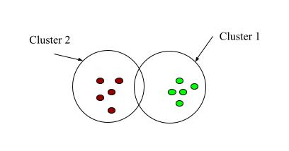
Fig 1: Clustering

As the name suggests, clustering literally means grouping similar things together and keeping apart different things. Clustering in machine learning groups similar data points keeping apart the different data points. 

As mentioned above, many times you would encounter unlabeled data in the real world, and getting the data labeled from experts is time-consuming and costly. In such scenarios, it is not possible to apply supervised machine learning algorithms.

However, the unlabeled data is not a waste as there can be some useful patterns hidden in the data. The unsupervised machine learning algorithms exploit this property of unlabeled data and try to find the hidden properties.  

One of the many unsupervised algorithms is clustering. It is the most basic form of unsupervised learning. People usually learn about unsupervised learning through clustering. Clustering is widely used in the real world to detect anomalies, identify malfunctioning, study genetics patterns, etc. 

Clustering algorithms vary in how different algorithms perceive the similarity and dissimilarity in the data. They also vary in the way each of them separates the clusters from each other. On the basis of these approaches, clustering can be broadly classified into four different types. Most of the algorithms fall under one of these categories. The next section discusses these categories one by one.

Types of Clustering

Given below are four different kinds of clustering techniques that handle all types of data differently. Let us understand each one of them.

Density-based Clustering

Density-based clustering relies on the fact that similar data points exist in proximity thus forming high-density regions separated by low-density regions. The density-based clustering algorithms try to find such high-density regions and call each of such regions the clusters. 

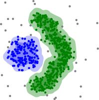
Fig 2: Density-based clustering (sourced from Wikipedia)

Let Eps be the maximum radius of a cluster. Let ‘minPts’ be the minimum number of data points in a cluster. Then,

NEPS = {k ϵ D, dist(i, k) <= EPS} where D is the dataset of all data points.

All the data points belonging to NEPS are said to be directly density reachable. 

The salient features of density-based clustering are as follows.

• The density-based clustering can form arbitrarily shaped clusters. It is not restricted to any particular shape.
• This method does not try to assign the outliers to the clusters thus providing an effective means of outlier analysis as well.
• You can define the density parameters.
• Examples of density-based clustering algorithms are DBSCAN and OPTICS discussed later in this article.

Distribution-based clustering

The distribution-based clustering method takes into account the distribution of the dataset. Each data point has a probability of belonging to a cluster. The probability decreases as the distance of the data point increase from the centroid of the cluster.

The distribution-based clustering is a soft clustering method that defines no hard boundaries between the clusters. However, you can explicitly make such an algorithm to perform the hard clustering by defining the rule that must be followed to belong to a cluster. For example, you can set a threshold probability or explicitly place the point to a cluster with the highest probability.

However, this type of clustering algorithm is useful when you have an idea of the distribution of your data. Otherwise, it is better to go with some different type of algorithm. 

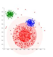
Fig 3: Distribution-based clustering (sourced from Wikipedia)

Centroid-based clustering

Centroid-based clustering is one of the most commonly used clustering techniques. It is probably the first type of clustering algorithm that you might have come across in the journey of learning clustering. In centroid-based clustering, the data points are assigned to clusters based on their distance from the cluster centroid. 

One of the most popular clustering algorithms, k-means clustering, is a centroid-based algorithm. It is efficient and fast but is sensitive to outliers and the results may vary depending on the initial parameters given to the algorithm.

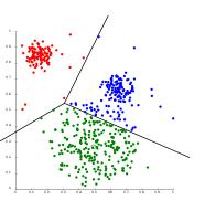
Fig 4: Centroid-based clustering (sourced from Wikipedia)

Hierarchical Clustering

Hierarchical clustering is a tree-based clustering method where a tree of clusters is formed from the given data. This type of clustering is more suited for data where a natural hierarchy is found such as taxonomies. This type of clustering forms well-organized clusters but it is more restrictive in nature than other methods.

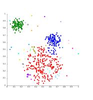
Fig 5: Hierarchical clustering (sourced from Wikipedia)

Other Classifications of Clustering Algorithms

The clustering algorithms can also be differentiated on the following basis.

Hard Clustering and Soft Clustering

• Hard Clustering: While clustering the data, if each of the data points belongs to a single specific cluster, then this type of clustering is known as hard clustering. Each data point can either belong to a cluster or does not belong to it. There is no probability involved in the existence of a data point in a cluster. Therefore, there is a hard boundary between different clusters.
• Soft Clustering: Soft clustering is a fuzzy clustering method in which the existence of a data point in a cluster is defined in terms of probability. A data point exists in different clusters with different probabilities, unlike hard clustering. Therefore, there is no hard boundary between clusters. 

Monothetic Clustering and Polythetic Clustering

• Monothetic Clustering: In this type of clustering, the cluster members have some common properties. Data is divided among different clusters on the basis of the values of a common feature.
• Polythetic Clustering: In this type of clustering, the cluster members exhibit some degree of similarity but may not have a common property. The cluster members are assigned based on the degree of similarity between the combination of a set of features.

Popular Clustering Algorithms

There are a number of popular clustering algorithms available that you can use for different use cases. These algorithms vary in the manner they approach the clustering. Each algorithm has its own pros and cons. Let us understand some of the most popular clustering algorithms with the help of code.

Library installation

Throughout this article, we will use the popular scikit-learn library to implement the different clustering algorithms in Python. We will also generate a random dataset of 1000 samples using the scikit-learn dataset’s ‘make_classification()’ method to feed to the clustering algorithm.

Therefore you must install the scikit-learn library in your system using the following command:

$ pip install scikit-learn

You must also have the numpy and the matplotlib library installed so that the data can be handled and viewed. You can do so by executing the following command:

$ pip install numpy
$ pip install matplotlib

K-means Clustering

K-means clustering is one of the most popular unsupervised machine learning algorithms. People are often introduced to clustering using K-mean clustering. The working of k-means clustering can be understood in simple steps given below.

• The k-means clustering algorithm accepts the number of clusters, k, as an argument.
• The ‘means’ in k-means essentially refers to averaging the data by finding the centroids.
• The algorithm starts with the random centroids which serve as the beginning points for clusters. The centroids can be real data points or imaginary locations. 
• It then re-calculates the cluster centroids through each iteration. 

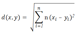
The distance measure used in the k-means clustering is often the Euclidean distance which can be calculated as given below.

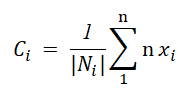
The algorithm re-calculates the centroid of each cluster by averaging all the data points of the clusters.

The algorithm stops when,

• The clustering has been completed, therefore, there is no change in the values of the centroids.
• The number of iterations has been reached.

Let us walk through the Python code for k-means clustering.

import numpy as np
from sklearn.datasets import make_classification
from sklearn.cluster import KMeans
from matplotlib import pyplot

# 2 features, 2 informative, 0 redundant, 1 cluster per class
X, y = make_classification(n_samples=1000, n_features=2, n_informative=2,
                           n_redundant=0, n_clusters_per_class=1, random_state=10) 

# 2 clusters
m = KMeans(n_clusters=2) 
# fit the model
m.fit(X)
# predict the cluster for each data point
p = m.predict(X) 
# unique clusters
cl = np.unique(p)
# plot the data points and cluster centers
for c in cl:
    r = np.where(c == p)
    pyplot.title('K-means (No. of Clusters = 3)')
    pyplot.scatter(X[r, 0], X[r, 1])
# show the plot
pyplot.show()

Output:

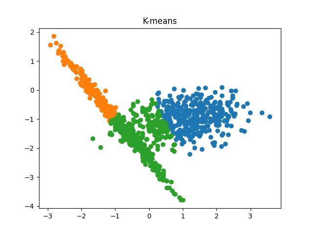
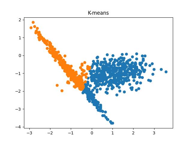
Fig 6: K-means clustering results when the number of clusters passed to the algorithm are 2 and 3, respectively.

You can check this tutorial where we performed image segmentation using K-means clustering.

Mini Batch K-means Clustering

Mini batch k-means clustering is a variant of k-means clustering. In each iteration, the algorithm fetches a predefined number of random samples from the dataset and stores them in the memory. These samples are then used to update the clusters and their centroids until the algorithm converges such that there is no significant change in the clusters. 

The advantages of the K-means mini-batch algorithm are given below.

• The algorithm does not store the complete dataset in the memory.
• At each iteration, the algorithm only calculates the distance between cluster centroids and the samples in a mini-batch.

Therefore, the mini-batch k-means algorithm might significantly outperform the traditional k-means clustering algorithm. 

Let us implement the mini-batch k-means clustering algorithm using the scikit-learn library in Python.

import numpy as np
from sklearn.datasets import make_classification
from sklearn.cluster import MiniBatchKMeans
from matplotlib import pyplot

X, y = make_classification(n_samples=1000, n_features=2, n_informative=2,
                           n_redundant=0, n_clusters_per_class=1, random_state=10)
# 3 clusters
m = MiniBatchKMeans(n_clusters=3) 
# fit the model
m.fit(X)
# predict the cluster for each data point
p = m.predict(X) 
# unique clusters
cl = np.unique(p)
# plot the data points and cluster centers
for c in cl:
    r = np.where(c == p)
    pyplot.title('Mini Batch K-means')
    pyplot.scatter(X[r, 0], X[r, 1])
# show the plot
pyplot.show()

Output:

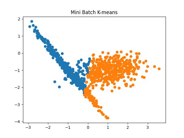
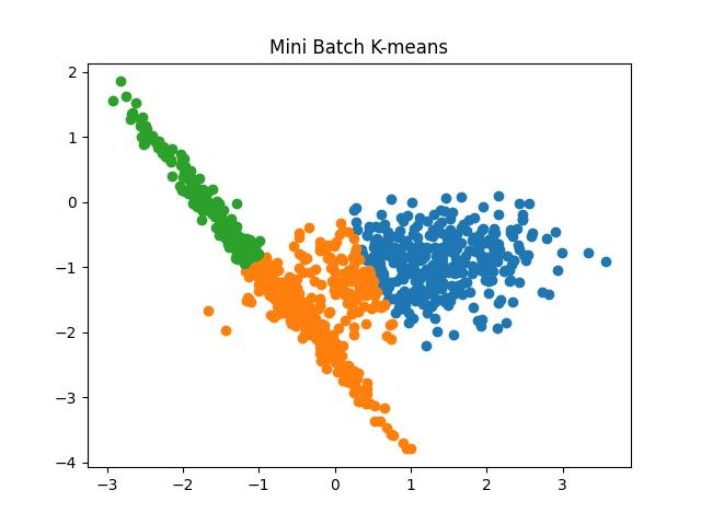
Fig 7: Mini Batch K Means algorithm results for the number of clusters as 2 and 3, respectively.

Comparison between the Time Taken by K-means and Mini-Batch K-means Algorithm

Let us perform an observational analysis of the time taken by K-means clustering and mini-batch K-means clustering algorithm to cluster the data.

import numpy as np
from sklearn.datasets import make_classification
from sklearn.cluster import MiniBatchKMeans
from sklearn.cluster import KMeans
from matplotlib import pyplot
import timeit

X, y = make_classification(n_samples=1000, n_features=2, n_informative=2,
                           n_redundant=0, n_clusters_per_class=1, random_state=10)
# start timer for Mini Batch K-Means
t1_mkm = timeit.default_timer() 
m = MiniBatchKMeans(n_clusters=2)
m.fit(X)
p = m.predict(X)
# stop timer for Mini Batch K-Means
t2_mkm = timeit.default_timer()
# start timer for K-Means
t1_km = timeit.default_timer()
m = KMeans(n_clusters=2)
m.fit(X)
p = m.predict(X)
# stop timer for K-Means
t2_km = timeit.default_timer()
# print time difference
print("Time difference between Mini Batch K-Means and K-Means = ",
      (t2_km-t1_km)-(t2_mkm-t1_mkm))

Output:

Time difference between Mini Batch K-Means and K-Means =  0.024629213998196064

Affinity Propagation

You have already seen that with K-means you need to specify the number of clusters beforehand. If you do not have knowledge of the number of clusters that might be existing in the data, you might want to choose the affinity propagation algorithm rather than K-means as it does not need any such parameters. For the same reason, this algorithm has gained popularity.

The algorithm proceeds in the following manner.

• All the data points are set as potential exemplars in the beginning.
• The data points send messages to all other data points and receive messages from all other data points.
• The point then decides, on the basis of the messages received, the point to which it would like to associate itself.
• This decision is then sent to the sender of the initial message informing its availability.
• The point that sends the message of its availability then becomes the exemplar to the sender of the original message.
• All the data points that have the same exemplar are associated with the same cluster.

The algorithm calculates the similarity matrix, responsibility matrix, availability matrix, and criterion matrix to come up with the clusters. For details on the algorithm, you can visit here.

Let us see the example of clustering using Affinity Propagation in Python:

import numpy as np
from sklearn.datasets import make_classification
from sklearn.cluster import AffinityPropagation
from matplotlib import pyplot

X, y = make_classification(n_samples=1000, n_features=2, n_informative=2,
                           n_redundant=0, n_clusters_per_class=1, random_state=10)

# initialize the model
m = AffinityPropagation(damping=0.9)
# fit the model
m.fit(X)
# predict the cluster for each data point
p = m.predict(X)
# unique clusters
cl = np.unique(p)
# plot the data points and cluster centers
for c in cl:
    r = np.where(c == p)
    pyplot.title('Affinity Propagation Clustering')
    pyplot.scatter(X[r, 0], X[r, 1])
# show the plot
pyplot.show()

Output:

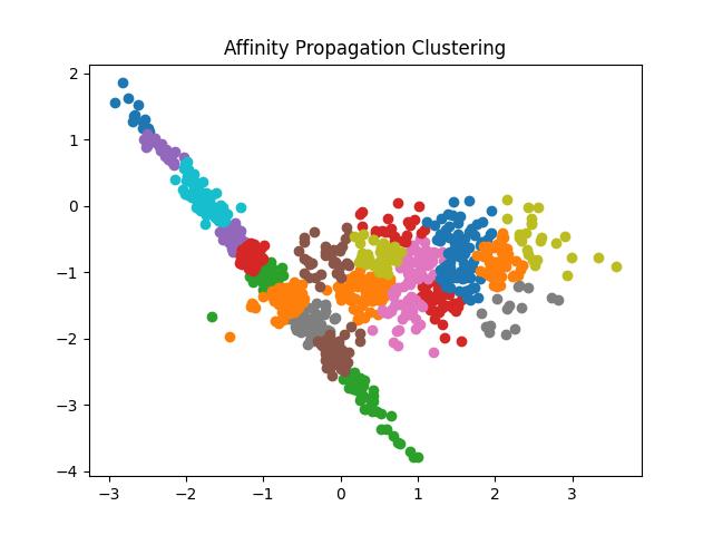
Fig 8: Result of Affinity Propagation clustering algorithm

DBSCAN Clustering Algorithm

The K-means algorithm is a powerful and popular clustering algorithm. But the K-means algorithm is sensitive to outliers as it eventually places all the data points into some cluster. Due to this, the outliers may significantly affect the final clusters. Yet another problem with the k-means algorithm is that you must provide the number of clusters to the algorithm. But many times you would not have that knowledge. 

DBSCAN (Density-Based Spatial Clustering of Applications with Noise) mitigates the aforementioned shortcomings greatly. The advantages of the DBSCAN algorithm as given below.

• You do not need to provide the number of clusters to the algorithm. It determines that on its own.
• DBSCAN algorithm can produce arbitrarily shaped clusters.
• It is much lesser sensitive to outliers. DBSCAN does not forcefully assign all data points to clusters.

The idea behind the DBSCAN algorithm is that similar data points are located in dense regions separated by regions of lower density. It, therefore, lies in the category of density-based clustering algorithms. The algorithm needs two parameters as given below.

• minPts: The minimum number of points needed to label a region as a cluster. Therefore you can control the density of your clusters.
• Epsilon: It signifies the distance that makes two points close to each other. You can control the sensitivity to outliers through these parameters.

There is a concept of connectivity and reachability in the DBSCAN algorithm. Reachability indicates whether a data point can be reached from another data point directly or indirectly whereas connectivity indicates if two data points lie in the same cluster.

On the basis of these measures, you can classify the points as follows.

• Core point: A point is said to be a core point if there exists at least ‘minPts’ number of data points within the ‘epsilon’ radius from the point.
• Border point: A point is a border point if there are less than ‘minPts’ points within its ‘epsilon’ radius but it is reachable from some other core point.
• Outlier: A point that is neither a core point nor a border point is called an outlier.

You can read more about the process of the DBSACN algorithm here.

Let us take a look at the implementation of the DBSCAN algorithm in Python:

import numpy as np
from sklearn.datasets import make_classification
from sklearn.cluster import DBSCAN
from matplotlib import pyplot

X, y = make_classification(n_samples=1000, n_features=2, n_informative=2,
                           n_redundant=0, n_clusters_per_class=1, random_state=10)
# init the model
m = DBSCAN(eps=0.05, min_samples=10)
# predict the cluster for each data point after fitting the model
p = m.fit_predict(X) 
# unique clusters
cl = np.unique(p)
# plot the data points and cluster centers
for c in cl:
    r = np.where(c == p)
    pyplot.title('DBSCAN Clustering')
    pyplot.scatter(X[r, 0], X[r, 1])
# show the plot
pyplot.show()

Output:

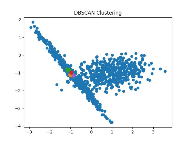
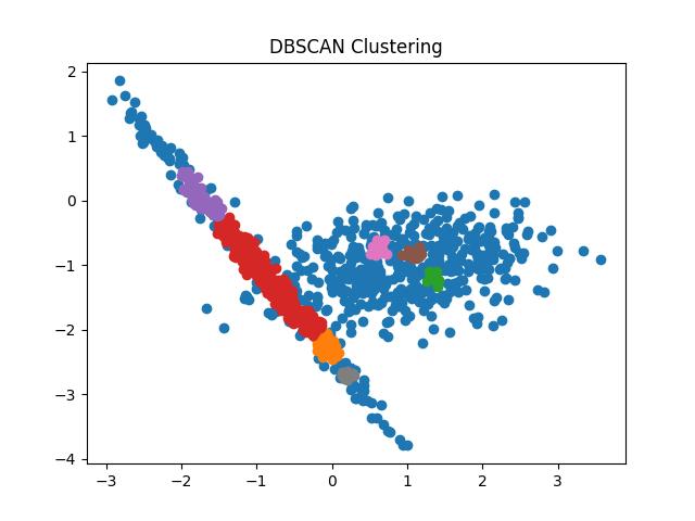
Fig 9: DBSCAN clustering result with eps = 0.05 and 0.1 respectively

OPTICS

OPTICS (Ordering Points To Identify Clustering Structure) can be termed as a successor of the DBSCAN algorithm. It is yet another density-based clustering algorithm that separates the clusters on the basis of the density of data points.

The DBSCAN algorithm assumes that the clusters are of fixed density which acts as a weakness of the algorithm. On the other hand, OPTICS allows clusters of varying densities. The OPTICS algorithm adds two more concepts to the DBSCAN algorithm as given below.

• Core distance: The core point to be classified as the core point should lie within the core distance. For a point that is not a core point, this variable is undefined.
• Reachability distance: The reachability distance between two core data points a and b is the maximum distance between a and b and the core distance of a.

You can read more about the OPTICS algorithm here. Let us see the example code of the OPTICS algorithm in Python:

import numpy as np
from sklearn.datasets import make_classification
from sklearn.cluster import OPTICS
from matplotlib import pyplot

X, y = make_classification(n_samples=1000, n_features=2, n_informative=2,
                           n_redundant=0, n_clusters_per_class=1, random_state=10)

# init the model
m = OPTICS(eps=0.5, min_samples=10)
# predict the cluster for each data point after fitting the model
p = m.fit_predict(X)
# unique clusters
cl = np.unique(p)
# plot the data points and cluster centers
for c in cl:
    r = np.where(c == p)
    pyplot.title('OPTICS Clustering')
    pyplot.scatter(X[r, 0], X[r, 1])
# show the plot
pyplot.show()

Output:

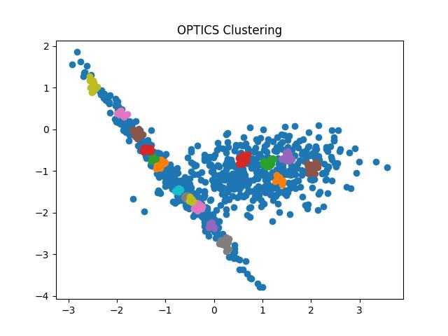
Fig 10: OPTICS clustering result with eps = 0.9 and 0.5 respectively

BIRCH

BIRCH (Balance Iterative Reducing and Clustering Hierarchies) is a hierarchical clustering algorithm. The algorithm first generates a summary of the large dataset preserving most of the information as possible. It then forms the clusters from the summarized data. For this reason, BIRCH is exclusively used for large datasets. 

However, the major drawback of BIRCH is that it can not handle categorical attributes. It is designed to handle only metric attributes. 

The BIRCH algorithm is a two-step algorithm. It works by first building the CF (Clustering Feature) tree and then performing the global clustering. BIRCH attempts to reduce the usage of memory by producing the CF tree from the density regions. Each entry of the CF tree consists of three parameters as given below.

where,

N = number of data elements in the cluster,

LS = Linear sum of all data elements in the cluster, and

SS = Squared sum of all data elements in the cluster.

Once the tree is formed the algorithm moves to the next step i.e. global clustering.

The algorithm accepts three parameters to perform the clustering. These parameters are given below.

• Threshold: It is the maximum number of data elements that the leaf node of the CF tree can hold in a sub-cluster.
• Branching Factor: It is the maximum number of sub-clusters in each node of the CF tree.
• Number of Clusters: This parameter signifies the total number of clusters that the algorithm produces after the final result i.e. after the global clustering. If this parameter is set to None, the algorithm returns intermediate clusters without performing the global clustering. 

If you are interested in the paper from the authors of BIRCH you can visit here.

Let us take a look at the clustering using the BIRCH algorithm in Python:

import numpy as np
from sklearn.datasets import make_classification
from sklearn.cluster import Birch
from matplotlib import pyplot

X, y = make_classification(n_samples=1000, n_features=2, n_informative=2,
                           n_redundant=0, n_clusters_per_class=1, random_state=10)
# init the model with 2 clusters
m = Birch(threshold=0.05, n_clusters=2)
# predict the cluster for each data point after fitting the model
p = m.fit_predict(X) 
# unique clusters
cl = np.unique(p)
# plot the data points and cluster centers
for c in cl:
    r = np.where(c == p)
    pyplot.title('Birch Clustering')
    pyplot.scatter(X[r, 0], X[r, 1])
# show the plot
pyplot.show()

Output:

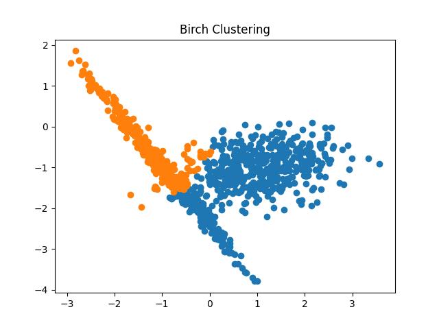
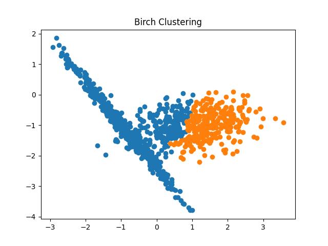
Fig 11: BIRCH Clustering algorithm result with different thresholds

Agglomerative Clustering

Agglomerative clustering is perhaps the most basic and commonly used hierarchical clustering algorithm. The algorithm creates the tree from the dataset by merging similar data points into one cluster until all data points are merged into a single cluster. The algorithm works as given below.

• The algorithm starts by considering all the data points as different clusters.
• Two clusters that are similar according to the similarity metric are merged into a single cluster.
• The second step is repeated until all the data points have been merged into a single cluster.

The resultant tree produced by the algorithm is called a dendrogram. As you might have noticed, Agglomerative Clustering produces the tree in a bottom-up manner. Yet another algorithm called the Divisive Clustering algorithm produces the tree in a top-down manner.

The measure of distance is important when you are working with hierarchical clustering algorithms. You can measure the distance between two clusters using various linkage methods as given below.

• Single linkage: It denotes the shortest distance between the closest data points of two clusters. 

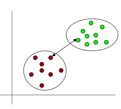
Fig 12: Single linkage

• Complete linkage: It denotes the longest distance between the data points of two clusters. 

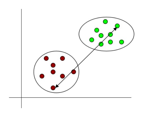
Fig 13: Complete linkage

• Average linkage: As the name suggests, it is the average of all pair-wise distances of data points of two clusters.
• Centroid linkage: It is the distance between centroids of two clusters.

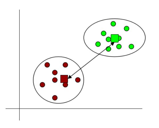
Fig 14: Centroid linkage

Let us take a look at the code of Agglomerative Clustering in Python:

import numpy as np
from sklearn.datasets import make_classification
from sklearn.cluster import AgglomerativeClustering
from matplotlib import pyplot

X, y = make_classification(n_samples=1000, n_features=2, n_informative=2,
                           n_redundant=0, n_clusters_per_class=1, random_state=10)
# init the model with 3 clusters
m = AgglomerativeClustering(n_clusters=3)
# predict the cluster for each data point after fitting the model
p = m.fit_predict(X) 
# unique clusters
cl = np.unique(p)
# plot the data points and cluster centers
for c in cl:
    r = np.where(c == p)
    pyplot.title('Agglomerative Clustering')
    pyplot.scatter(X[r, 0], X[r, 1])
# show the plot
pyplot.show()

Output:

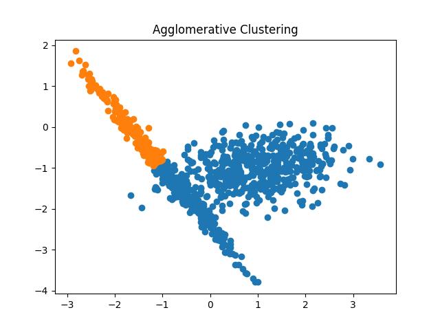
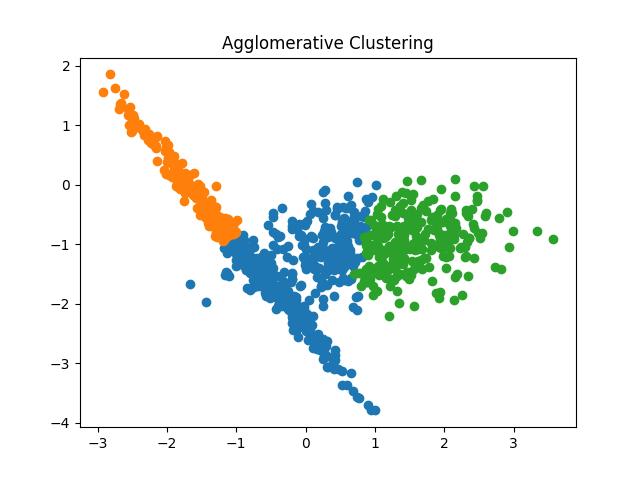
Fig 15: Agglomerative Clustering results with the number of clusters as 2 and 3 respectively

Mean-Shift Clustering

The Mean-Shift algorithm works by shifting the centroid of the clusters towards the regions of higher density successively in each iteration. The algorithm discovers the blobs of data points in density regions. It is a centroid-based algorithm that chooses the candidates for centroids and keeps updating them until no more updation happens.

You can trace the working of the algorithm by following the given steps.

• The first step is to create a sliding window cluster for every data element in the dataset.
• In each iteration, the centroid of the sliding window is updated and shifted towards the regions of high density. These centroids are meant to be the mean of data points of the respective sliding window.
• The second step is repeated until no more regions of higher density are discovered.
• In the post-processing step, the sliding windows are selected by deleting the overlapping sliding windows. If multiple sliding windows are overlapping, the algorithm selects the window of the highest density and deletes other windows.
• Finally, the clusters are formed from the sliding windows.

The mean shift algorithm is based on the Kernel Density Estimation (KDE) where each data point acts as a probability density function. Since the algorithm shifts the window towards regions of high density, it is also termed the hill-climbing algorithm.

The mean shift algorithm produces great results with spherical-shaped data. One of the main advantages of this algorithm is that you do not need to provide the number of clusters as the initialization parameter as in k-means clustering. Also, the output of the algorithm is not biased toward the initialization parameters.

However, the mean shift algorithm is not highly scalable as it needs multiple searches to search for the nearest neighbors in each window shift operation. You can learn more about the algorithm from the paper published by its authors.

Let us take a look at the mean shift algorithm in Python:

import numpy as np
from sklearn.datasets import make_classification
from sklearn.cluster import MeanShift
from matplotlib import pyplot

X, y = make_classification(n_samples=1000, n_features=2, n_informative=2,
                           n_redundant=0, n_clusters_per_class=1, random_state=10)
# init the model
m = MeanShift()
# predict the cluster for each data point after fitting the model
p = m.fit_predict(X)
# unique clusters
cl = np.unique(p)
# plot the data points and cluster centers
for c in cl:
    r = np.where(c == p)
    pyplot.title('Mean Shift Clustering')
    pyplot.scatter(X[r, 0], X[r, 1])
# show the plot
pyplot.show()

Output:

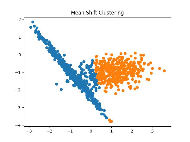
Fig 16: Mean Shift Clustering Result

Spectral Clustering

The spectral clustering algorithm has been creating a buzz in recent times due to its simplicity, efficiency, ability to be solved by linear algebra, and performance in comparison to the classic clustering algorithms. 

The spectral clustering algorithm is very often used in exploratory data analysis and dimensionality reduction of complex and multidimensional data. The algorithm takes the graphical approach to clustering where it identifies data points that are connected or are immediately next to each other. Once such nodes are identified, these are used to form clusters in lower dimensions.

One of the advantages of spectral clustering is that it makes no assumptions about the form of the cluster. Therefore, it is more accurate. However, the algorithm is less scalable for large datasets as the complexity increases and the accuracy decreases. The steps in spectral clustering are given below.

• The algorithm first creates a distance matrix from data points.
• It then creates an affinity matrix from the distance matrix and computes the degree matrix and Laplacian matrix.
• The algorithm then generates the eigenvalues and eigenvectors of the Laplacian matrix.
• Finally, a matrix is formed from eigenvectors with ‘k’ largest eigenvalues. The algorithm then normalizes the vectors.
• In the last step, it forms clusters from data points in k-dimensional space.

 Let us see the code example of spectral clustering in Python:

import numpy as np
from sklearn.datasets import make_classification
from sklearn.cluster import SpectralClustering
from matplotlib import pyplot

X, y = make_classification(n_samples=1000, n_features=2, n_informative=2,
                           n_redundant=0, n_clusters_per_class=1, random_state=10)
# init the model with 3 clusters
m = SpectralClustering(n_clusters=3)
# predict the cluster for each data point after fitting the model
p = m.fit_predict(X)
# unique clusters
cl = np.unique(p)
# plot the data points and cluster centers
for c in cl:
    r = np.where(c == p)
    pyplot.title('Spectral Clustering')
    pyplot.scatter(X[r, 0], X[r, 1])
# show the plot
pyplot.show()

Output:

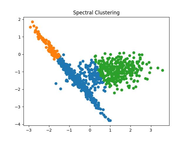
Fig 17: Spectral Clustering result with the number of clusters as 2 and 3 respectively

Gaussian Mixture Model

The gaussian mixture model is based on the gaussian distribution of the data. The model tries to fit different Gaussian models to the data and learn the parameters such as mean and variance of distributions. The algorithm then uses these parameters to calculate the probabilities of the existence of the data points in different clusters.

The gaussian mixture model is similar yet different to the k-means clustering. To be exact, it has two major advantages over the k-means clustering algorithm.  

• The first advantage is that the Gaussian mixture model takes into account the variance of the data while k-means does not.
• Second, the k-means algorithm is a hard clustering algorithm where a data point either exists in a cluster or does not belong to the cluster. However, the Gaussian mixture model gives probabilities of the existence of a data point in a cluster. Therefore, it is a soft clustering method.

The Gaussian mixture model works as follows.

• The algorithm first initializes parameters mean, covariance, and mixing coefficients randomly. 
• It then computes the coefficient assignment values for all Gaussians.
• Estimate the parameters again using the computed coefficient assignment. 
• The algorithm then computes the log-likelihood function and defines some rules about the convergence criterion. 
• If the log-likelihood value converges, it then stops and produces the clusters, otherwise, the algorithm begins again from step 2.

Let us take a look at the Python code of the gaussian mixture model clustering:

import numpy as np
from sklearn.datasets import make_classification
from sklearn.mixture import GaussianMixture
from matplotlib import pyplot

X, y = make_classification(n_samples=1000, n_features=2, n_informative=2,
                           n_redundant=0, n_clusters_per_class=1, random_state=10)
# init the model with 2 components
m = GaussianMixture(n_components=2)
# predict the cluster for each data point after fitting the model
p = m.fit_predict(X)
# unique clusters
cl = np.unique(p)
# plot the data points and cluster centers
for c in cl:
    r = np.where(c == p)
    pyplot.title('Gaussian Mixture Clustering')
    pyplot.scatter(X[r, 0], X[r, 1])
# show the plot
pyplot.show()

Output:

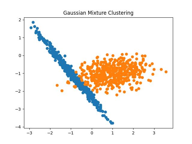
Fig 18: Gaussian Mixture Model clustering result

Metrics for Evaluation of Clustering Algorithms

Once you have obtained the clusters from your clustering algorithm, you would want to evaluate the results. There are certain metrics to evaluate the clustering results. Let us take a tour of each one of them.

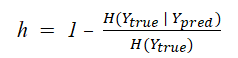
Homogeneity Score

The homogeneity score evaluates the clusters on the basis of the class labels of the cluster members. If all data points in all the clusters belong to the same class, it is said to satisfy the homogeneity condition. 

The homogeneity score lies between 0 and 1 where 0 is completely non-homogenous and 1 is perfectly homogenous. You can calculate the homogeneity score by using the equation given below.

Completeness Score

If all the data points of a class lie in the same clusters, then the clustering results are said to satisfy the completeness property. The completeness score can be computed using the formula given below.

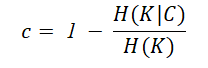
The completeness score also lies between 0 and 1 where 1 denotes perfect completeness and 0 means no completeness at all.

V Measure Score

The v-measure score establishes the goodness of the clustering algorithm. It is the harmonic mean between the completeness score and the homogeneity score. The formula for the v-measure score is given below.

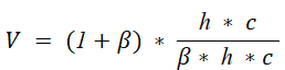
The v-measure score lies between 0 and 1 where 1 denotes that the clustering is perfect. You can get these metrics of the clustering algorithms using the scikit-learn library’s inbuilt functions as given in the example below.

from sklearn import metrics

y_true = [5, 3, 5, 4, 4, 5]
y_pred = [3, 5, 5, 4, 3, 4]
# homogeneity: each cluster contains only members of a single class.
print(metrics.homogeneity_score(y_true, y_pred))
# completeness: all members of a given class are assigned to the same cluster.
print(metrics.completeness_score(y_true, y_pred))
# v-measure: harmonic mean of homogeneity and completeness
print(metrics.v_measure_score(y_true, y_pred))

Output:

0.3146685210384134
0.28969008214284747
0.30166311599620416

Use Cases of Clustering

The data produced by real-world applications and processes are largely unlabeled. Therefore clustering has a large number of practical use cases. In general, when you have unlabeled data and there is a chance of finding some hidden partitioning in the data, you may consider clustering as your first approach. Some of the practical use cases of clustering are listed below.

• Customer Segmentation: The corporates use clustering to obtain the customer segmentation results so that the marketing strategies can be formulated effectively.
• Biology: Genetics are studied using clustering in biology.
• Medicine: Clustering helps in finding meaningful results in drug interactions and drug manufacturing.
• Image compression: Clustering helps to preserve the information while reducing the dimensionality of the image. 
• Library: The books on different topics and subjects in the library are managed using clustering.
• Document analysis: The research papers and other documents can be grouped together on the basis of the similarity between them using the clustering methods. 

Best Clustering Algorithm and Things to Keep in Mind

After going through different clustering algorithms you might be wondering which algorithm is the best clustering algorithm. The answer to your question is that there is no one perfect clustering algorithm that fits all the needs.

Different clustering algorithms have different advantages and disadvantages. Some are simple while others are complex, some need initialization parameters while others don’t, some scale well while others do not scale so well, and so on. 

Therefore, the choice of clustering algorithm depends on your use case. However, keep the following points in mind while choosing the algorithm:

• If your application needs fast results, you must choose an algorithm of lower time complexity.
• If you do not know the distribution of the data, you must avoid distribution-based clustering algorithms.
• If you have a very large data set you should select an algorithm that scales well.

Conclusion

The article discussed the categories of clustering algorithms, most of the popular clustering algorithms, and the metrics to evaluate these algorithms. You have also seen the practical use cases of clustering and the points to remember while choosing the algorithm. By now, you have hopefully gained sufficient knowledge to use clustering in your application effectively.

Learn also: How to Use K-Means Clustering for Image Segmentation using OpenCV in Python.

Happy coding ♥

Let our Code Converter simplify your multi-language projects. It's like having a coding translator at your fingertips. Don't miss out!

View Full Code Auto-Generate My Code

Read Also

Comment panel