Dimensionality Reduction Using Feature Selection in Python

Adrien Payong · 10 min read · Updated jun 2022 · Machine Learning

Before we get started, have you tried our new Python Code Assistant? It's like having an expert coder at your fingertips. Check it out!

Introduction

Feature selection is the process of choosing a subset of features from the dataset that contributes the most to the performance of the model, and this without applying any type of transformation to it.

Feature selection is broken down into three categories: filter, wrapper, and embedding. Filter techniques examine the statistical properties of features to determine which ones are the best. Wrapper approaches employ trial and error to select the subset of features that provide the most accurate models.

In the end, embedding techniques choose the optimal feature subset during or as an extension of the training phase of a learning algorithm. Ideally, this tutorial would cover all three approaches.

A deeper look into particular learning algorithms makes it harder to describe embedded approaches prior to a deeper study into those algorithms. Consequently, we will solely discuss filter and wrapper feature selection techniques.

The diagram below depicts the various types of feature selection.

featureselection 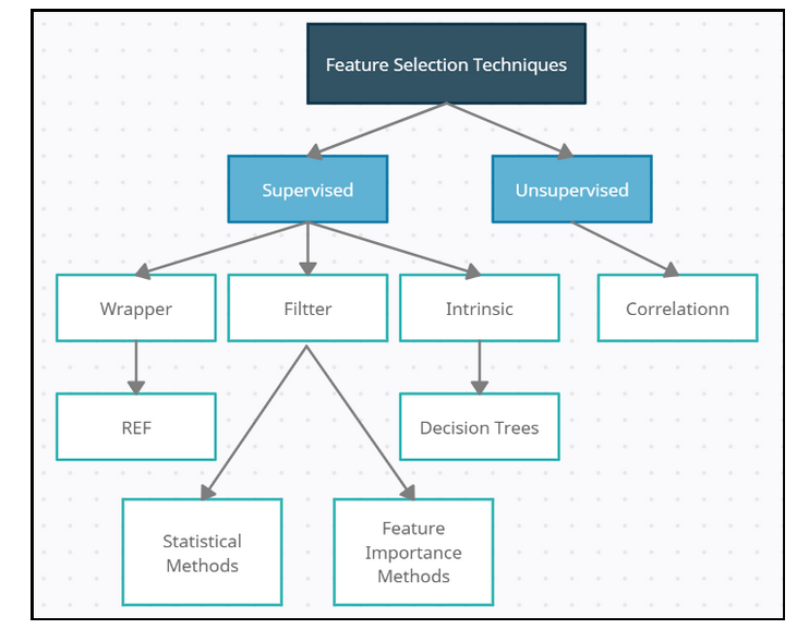Source: medium

Table of content:

Thresholding Numerical Feature Variance
Thresholding Binary Feature Variance
Handling Highly Correlated Features
Removing Irrelevant Features for Classification
Recursively Eliminating Features
Conclusion

Thresholding Numerical Feature Variance

Suppose that you want to exclude features with a low variance from a collection of numerical features. Variance thresholding (VT) is a fundamental method for selecting features. Based on the hypothesis that traits with low variance aren't as interesting (or valuable) as those with high variance, this approach was developed. First, the variance of each feature can be calculated through the following formula:

thresholding

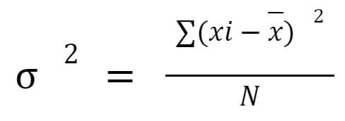
where x is the feature vector, xi is an individual feature value, and x̄ is the mean value of that feature. It removes any features whose variance does not meet that criterion.

It is important to remember two things while using VT: This variance is not centered, meaning it is in the feature's squared unit. This means that feature sets with multiple units (e.g., one feature is in years and another in dollars) will not operate with the VT.

Since the variance threshold must be manually set, we must rely on our own experience and expertise in making this choice (or use a model selection technique). You can follow the code below:

# Load libraries
# import data
iris = datasets.load_iris()
# Create features and target
features_i = iris.data
target_i = iris.target
# thresholder  creation
thresholder = VarianceThreshold(threshold=.4)
# high variance feature matrix creation
f_high_variance = thresholder.fit_transform(features_i)
# View high variance feature matrix
f_high_variance[0:3]

array([[5.1, 1.4, 0.2],
       [4.9, 1.4, 0.2],
       [4.7, 1.3, 0.2]])

Each feature's variance may be viewed using variances_.

# View variances
thresholder.fit(features_i).variances_

Output:

array([0.68112222, 0.18871289, 3.09550267, 0.57713289])

As the last point, variance thresholding will fail if the features are standardized (i.e., mean zero and unit variance).

# feature matrix stantardization
scaler = StandardScaler()
f_std = scaler.fit_transform(features_i)
# variance of each feature calculation
selection = VarianceThreshold()
selection.fit(f_std).variances_

array([1., 1., 1., 1.])

Thresholding Binary Feature Variance

Variance analysis may be used to pick the most useful categories, much as with numerical features. For Bernoulli random variables (binary features), the following formula is used to compute the variance:

Variance(x) = p(1 − p)

p is the observations proportion of class 1. Consequently, by adjusting p, we may delete features where the majority of observations are class one.

Suppose that a collection of binary categorical features has been collected, and we want to eliminate the features with low variance (i.e., likely containing little information). We will select attributes that have a Bernoulli random variable variance above a predetermined threshold:

# feature matrix creation with:
# for Feature 0: 80% class 0
# for Feature 1: 80% class 1
# for Feature 2: 60% class 0, 40% class 1
features_i = [[0, 2, 0],
[0, 1, 1],
[0, 1, 0],
[0, 1, 1],
[1, 0, 0]]
# threshold by variance
thresholding = VarianceThreshold(threshold=(.65 * (1 - .65)))
thresholding.fit_transform(features_i)

array([[2, 0],
       [1, 1],
       [1, 0],
       [1, 1],
       [0, 0]])

Handling Highly Correlated Features

If you have a feature matrix and feel that certain of the features are highly correlated, just check for highly correlated features using a correlation matrix. If there are highly correlated traits, try dropping one of them.

# Create feature matrix with two highly correlated features
features_m = np.array([[1, 1, 1],
[2, 2, 0],
[3, 3, 1],
[4, 4, 0],
[5, 5, 1],
[6, 6, 0],
[7, 7, 1],
[8, 7, 0],
[9, 7, 1]])
# Conversion of  feature matrix
dataframe = pd.DataFrame(features_m)
# correlation matrix creation
corr_m = dataframe.corr().abs()
# upper triangle selection
upper1 = corr_m.where(np.triu(np.ones(corr_m.shape),
k=1).astype(np.bool))
# For correlation greater than 0.85, Find index of feature columns
droping = [col for col in upper1.columns if any(upper1[col] > 0.85)]
# Drop features
dataframe.drop(dataframe.columns[droping], axis=1).head(3)

Highly correlated features are a common issue in machine learning. When two traits are strongly correlated, the information they provide is quite similar, and it is likely redundant to include both.

Removing one of the correlated features from the feature set solves the problem. As part of our approach, we first build up a correlation matrix that includes all features. We use the dataframe.corr() method and look at the correlation matrix's upper triangle to find pairs of highly correlated features and eliminate one feature from each of those pairs.

Removing Irrelevant Features for Classification

Suppose you want to remove a non-informative feature from a category target vector. You can calculate a chi-square statistic between each feature and the target vector if the features are categorical.

# Load data
iris_i = load_iris()
features_v = iris.data
target = iris.target
# categorical data coversion
features_v = features_v.astype(int)
# Selection of two features using highest chi-squared 
chi2_s = SelectKBest(chi2, k=2)
f_kbest = chi2_s.fit_transform(features_v, target)
# Show results
print("Original number of features:", features_v.shape[1])
print("Reduced number of features:", f_kbest.shape[1])

Original number of features: 4
Reduced number of features: 2

Determine the ANOVA F-value between each feature and the target vector if the features are quantitative.

# Selection of two features using highest F-values
f_selector = SelectKBest(f_classif, k=2)
f_kbest = f_selector.fit_transform(features_v, target)
# Pisplay results
print("Original number of features:", features_v.shape[1])
print("Reduced number of features:", f_kbest.shape[1])

Original number of features: 4
Reduced number of features: 2

SelectPercentile may be used to choose the top n percent of features instead of a specified number of features.

# Selection of top 65% of features 
f_selector = SelectPercentile(f_classif, percentile=65)
f_kbest = f_selector.fit_transform(features_v, target)
# Display results
print("Original number of features:", features_v.shape[1])
print("Reduced number of features:", f_kbest.shape[1])

Original number of features: 4
Reduced number of features: 2

The independence of two category vectors is investigated using chi-square statistics: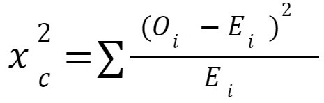

Chi square O_i is the number of observations in class i. E_i is the number of observations in class i, if we would predict if the feature and target vector are not related. A chi-squared statistic is a single value that informs you how much difference there is between your observed counts and the counts you would predict if there was no association in the population.

Calculating the chi-squared statistic between a feature and the target vector gives an assessment of independence between the two. If the target is unrelated to the feature variable, it is meaningless to us since it includes no information that may be used for classification. If the two features are strongly dependent, they are likely to be particularly informative for training our model.

Chi-squared statistics are used to choose features by determining how well each feature correlates with the target vector and then selecting the features using the best chi-square statistics.

The k option defines how many features we want to retain. To use chi-squared for feature selection, the target vector and features must both be categorical. We can employ the chi-squared approach if we have a numerical value that can be transformed into a categorical feature, and the chi-squared technique requires that all values be non-negative.
SelectKBest may be used to choose the most statistically significant features.
Additionally, f_classif may be used to compute the ANOVA F-value statistic for each feature and target vector when numerical features are available. F-value scores analyze whether or not the means of the numerical features are substantially different when we group them by the target vector.

Recursively Eliminating Features

You want to choose automatically the finest features. RFECV may be used to perform recursive feature elimination (RFE) with cross-validation (CV).

RFE is built on the idea of repeatedly training a model like linear regression or support vector machines that include parameters (also known as weights or coefficients). We incorporate all of the features in the model's first training. To eliminate a feature from a feature set, we look for the feature with the smallest parameter (noting that this presupposes that the features be either rescaled or standardized).

Adding a new concept called cross-validation (CV) is necessary for a better strategy. Obviously, how many features should we keep? Repeating this loop until only one feature remains is possible (in theory).

Cross-validation is used to determine the optimal amount of features to preserve during RFE. In RFE with CV, we employ cross-validation to test our model after each iteration. If CV demonstrates that our model improved after we removed a feature, we go to the next cycle. However, if CV indicates that our model deteriorated after we removed a feature, we reinstate that feature in the feature set and select those features as the best.

RFE with CV is implemented using the RFECV() class and includes a number of key parameters:

The estimator parameter specifies the kind of model to be trained (e.g., linear regression).
The step regression algorithm specifies the amount or fraction of features to be dropped throughout each loop.
The scoring parameter specifies the quality measure that will be used to assess our model during cross-validation.

# Load libraries
# Suppress an annoying but harmless warning
warnings.filterwarnings(action="ignore", module="scipy",
message="^internal gelsd")
#  features matrix, target vector, true coefficients
features_f, target_t = make_regression(n_samples = 10000,
n_features = 100,
n_informative = 2,
random_state = 1)
# linear regression creation
ols = linear_model.LinearRegression()
# Recursive features elimination
rfecv = RFECV(estimator=ols, step=2, scoring="neg_mean_squared_error")
rfecv.fit(features_f, target_t)
rfecv.transform(features_f)

array([[ 0.00850799,  0.7031277 ],
       [-1.07500204,  2.56148527],
       [ 1.37940721, -1.77039484],
       ...,
       [-0.80331656, -1.60648007],
       [ 0.39508844, -1.34564911],
       [-0.55383035,  0.82880112]])

Following the RFE process, we can have a better idea of how many features we should keep:

# Number of best features
rfecv.n_features_

We may additionally determine which of these traits should be retained:

# What the best categories ?
rfecv.support_

array([False, False, False, False, False,  True, False, False, False,
       False, False, False, False, False, False, False, False, False,
       False, False, False, False, False, False, False, False, False,
       False, False, False, False, False, False, False, False, False,
       False, False, False,  True, False, False, False, False, False,
       False, False, False, False, False, False, False, False, False,
       False, False, False, False, False, False, False, False, False,
       False, False, False, False, False, False, False, False, False,
       False, False, False, False, False, False, False, False, False,
       False, False, False, False, False, False, False, False, False,
       False, False, False, False, False, False, False, False, False,
       False])

We can even view the rankings of the features:

# We can even see how the features are ranked
rfecv.ranking_

array([16, 18, 43, 40, 13,  1, 26, 22, 44, 31, 23, 33, 22, 32, 14, 12, 35,
        2, 29, 11, 11, 41,  3, 37, 46, 34, 45, 48,  4, 12,  2, 49, 16, 10,
       40, 20, 14, 15,  5,  1, 21,  6, 45, 47, 29, 42, 17,  6,  7, 10, 24,
       41, 47, 19,  8,  8, 26, 43, 49, 46, 28, 19,  4, 24, 48,  3, 33, 42,
        5, 38, 27, 31, 50, 30,  9, 50, 17, 23,  7, 30, 34,  9, 28, 37, 20,
       13, 21, 25, 38, 39, 32, 39, 36, 36, 15, 27, 44, 35, 18, 25])

Conclusion

Feature selection is a critical phase in the development of machine learning models. It can shorten training time, simplify our models, make them easier to debug, and shorten the time to market for machine learning solutions.

Get the complete code here.

Learn also: Feature Selection using Scikit-Learn in Python

Happy coding ♥

Just finished the article? Why not take your Python skills a notch higher with our Python Code Assistant? Check it out!

View Full Code Auto-Generate My Code

Sharing is caring!

Comment panel

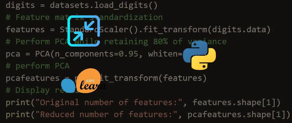
Got a coding query or need some guidance before you comment? Check out this Python Code Assistant for expert advice and handy tips. It's like having a coding tutor right in your fingertips!