How to Fine Tune ViT for Image Classification using Transformers in Python

Abdeladim Fadheli · 16 min read · Updated mar 2023 · Machine Learning · Computer Vision

Get a head start on your coding projects with our Python Code Generator. Perfect for those times when you need a quick solution. Don't wait, try it today!

Image classification is one of the most common tasks in computer vision and machine learning. It involves training a deep neural network to recognize and classify images into two or more predefined categories or classes.

As you may already know, image classification is currently used in many applications in the real-world, such as medical diagnosis (analyzing chest X-ray images, skin cancer, etc.), facial recognition, satellite image classification, quality control in manufacturing, and many more.

In a previous tutorial, we built a CNN-based image classifier from scratch using the Keras API. In this tutorial, you will learn how to finetune the state-of-the-art vision transformer (ViT) on your custom image classification dataset using the Huggingface Transformers library in Python.

ViT model is pre-trained on ImageNet-21k (14 million images, and 21,843 classes) at the 224x224 resolution, and fine-tuned on the ImageNet 2012 dataset (1 million images, 1,000 classes). It was introduced in the famous paper: An Image is Worth 16x16 Words: Transformers for Image Recognition at Scale.

If you're familiar with BERT, then ViT is quite similar but for images instead of text. The idea of the vision transformer architecture is that it splits the image into fixed-size patches, these patches are flattened and then lower-dimensional linear embeddings are created from these patches. This way, it behaves as if it's a sequence of text. The below figure shows the ViT architecture, taken from the original paper:

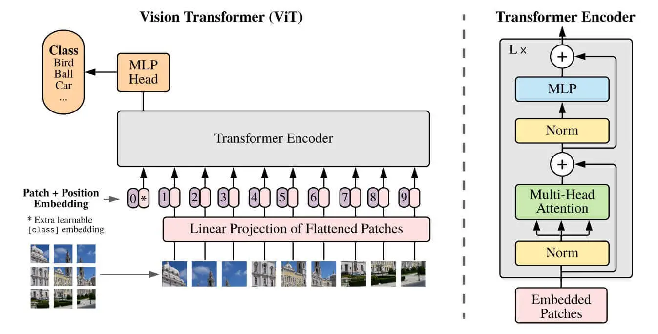Figure 1: The Vision Transformer (ViT) architecture

Table of content:

Getting Started
Loading our Dataset
Exploring the Dataset
Preprocessing the Data
Defining the Metrics
Training the Model
Performing Inference
Conclusion

Getting Started

To get started, let's install 🤗 transformers and PyTorch:

$ pip install torch transformers evaluate datasets

If you're not on Colab, then make sure to follow this guide to install PyTorch for your CUDA device and version.

We'll be using the 🤗 evaluate library to calculate the F1 and accuracy scores, and 🤗 datasets for loading our dataset.

Open up a new notebook and import the following:

import requests
import torch
from PIL import Image
from transformers import *
from tqdm import tqdm

device = "cuda" if torch.cuda.is_available() else "cpu"

If the CUDA is available, we set the device to "cuda", and "cpu" otherwise. It's not suggested to run the training on CPU as it'll take a very long time.

Next, let's initialize our model, which is the ViT base model, namely google/vit-base-patch16-224:

# the model name
model_name = "google/vit-base-patch16-224"
# load the image processor
image_processor = ViTImageProcessor.from_pretrained(model_name)
# loading the pre-trained model
model = ViTForImageClassification.from_pretrained(model_name)

We're also loading our image processor in the above code, as it'll be responsible for preprocessing the image before pushing it into the model. The preprocessing tasks are resizing the image to the appropriate resolution (224x224 in this case), and normalizing the pixel values. You can check the preprocessor config file here.

To be able to load images, I'm adding two helper functions for that:

import urllib.parse as parse
import os

# a function to determine whether a string is a URL or not
def is_url(string):
    try:
        result = parse.urlparse(string)
        return all([result.scheme, result.netloc, result.path])
    except:
        return False
    
# a function to load an image
def load_image(image_path):
    if is_url(image_path):
        return Image.open(requests.get(image_path, stream=True).raw)
    elif os.path.exists(image_path):
        return Image.open(image_path)

These are grabbed from the image captioning tutorial, is_url() checks whether a string is a URL, and the load_image() function takes the image path or URL and loads it. If it's a URL, it downloads it using the requests library.

Before diving into fine-tuning, let's try out the current model weights with some images. Before that, let's make a function that takes the model and image path or URL, and returns the predicted class:

def get_prediction(model, url_or_path):
  # load the image
  img = load_image(url_or_path)
  # preprocessing the image
  pixel_values = image_processor(img, return_tensors="pt")["pixel_values"].to(device)
  # perform inference
  output = model(pixel_values)
  # get the label id and return the class name
  return model.config.id2label[int(output.logits.softmax(dim=1).argmax())]

We load our image, preprocess it and perform inference on the pixel values. Finally, we perform the argmax() after the softmax() function to the model output logits, we use the model.config.id2label to convert the class ID into class name.

Let's try it now:

get_prediction(model, "http://images.cocodataset.org/test-stuff2017/000000000128.jpg")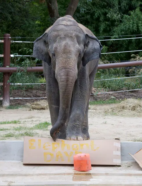

An elephant

Output:

Indian elephant, Elephas maximus

Loading our Dataset

🤗 Datasets makes it easy to upload your custom dataset to the 🤗 Datasets hub via either uploading your dataset or creating one. If you're worried about your dataset being public, you can make the choice to keep it private, while still using the datasets functionalities in code.

For this tutorial, I'm picking the food101 classification dataset, which consists of 101 food categories and a total of 101,000 images.

Let's load it:

from datasets import load_dataset

# download & load the dataset
ds = load_dataset("food101")

This will take a few minutes to download and load, as it's a 5GB file.

Alternatively, if you want to quickly load your custom dataset, then you can use the ImageFolder dataset builder. It does not require making a custom data loader, but your dataset structure should look like this:

folder/train/dog/golden_retriever.png
folder/train/dog/german_shepherd.png
folder/train/dog/chihuahua.png

folder/train/cat/maine_coon.png
folder/train/cat/bengal.png
folder/train/cat/birman.png

For instance, let me download and load a dataset from the skin cancer detection tutorial:

import requests
from tqdm import tqdm
import zipfile
import os

def get_file(url):
  response = requests.get(url, stream=True)
  total_size = int(response.headers.get('content-length', 0))
  filename = None
  content_disposition = response.headers.get('content-disposition')
  if content_disposition:
      parts = content_disposition.split(';')
      for part in parts:
          if 'filename' in part:
              filename = part.split('=')[1].strip('"')
  if not filename:
      filename = os.path.basename(url)
  block_size = 1024 # 1 Kibibyte
  tqdm_bar = tqdm(total=total_size, unit='iB', unit_scale=True)
  with open(filename, 'wb') as file:
      for data in response.iter_content(block_size):
          tqdm_bar.update(len(data))
          file.write(data)
  tqdm_bar.close()
  print(f"Downloaded {filename} ({total_size} bytes)")
  return filename

def download_and_extract_dataset():
  # dataset from https://github.com/udacity/dermatologist-ai
  # 5.3GB
  train_url = "https://s3-us-west-1.amazonaws.com/udacity-dlnfd/datasets/skin-cancer/train.zip"
  # 824.5MB
  valid_url = "https://s3-us-west-1.amazonaws.com/udacity-dlnfd/datasets/skin-cancer/valid.zip"
  # 5.1GB
  test_url  = "https://s3-us-west-1.amazonaws.com/udacity-dlnfd/datasets/skin-cancer/test.zip"
  for i, download_link in enumerate([valid_url, train_url, test_url]):
    data_dir = get_file(download_link)
    print("Extracting", download_link)
    with zipfile.ZipFile(data_dir, "r") as z:
      z.extractall("data")
    # remove the temp file
    os.remove(data_dir)

# comment the below line if you already downloaded the dataset
download_and_extract_dataset()

The dataset will be downloaded and extracted, and is structured like this:

data/train/melanoma/ISIC_0000002.jpg
data/train/melanoma/ISIC_0000004.jpg
data/train/melanoma/ISIC_0000013.jpg
...
data/test/nevus/ISIC_0012092.jpg
data/test/nevus/ISIC_0012095.jpg
data/test/nevus/ISIC_0012247.jpg
...

Therefore, I can simply load it using the below code:

from datasets import load_dataset

# load the custom dataset
ds = load_dataset("imagefolder", data_dir="data")
ds

Exploring the Dataset

Going back to the food101 dataset. Here's the output of ds:

DatasetDict({
    train: Dataset({
        features: ['image', 'label'],
        num_rows: 75750
    })
    validation: Dataset({
        features: ['image', 'label'],
        num_rows: 25250
    })
})

Let's see the labels:

labels = ds["train"].features["label"]
labels

Output:

ClassLabel(names=['apple_pie', 'baby_back_ribs', 'baklava', 'beef_carpaccio', 'beef_tartare', 'beet_salad', 'beignets', 'bibimbap', 'bread_pudding', 'breakfast_burrito', 'bruschetta', 'caesar_salad', 'cannoli', 'caprese_salad', 'carrot_cake', 'ceviche', 'cheesecake', 'cheese_plate', 'chicken_curry', 'chicken_quesadilla', 'chicken_wings', 'chocolate_cake', 'chocolate_mousse', 'churros', 'clam_chowder', 'club_sandwich', 'crab_cakes', 'creme_brulee', 'croque_madame', 'cup_cakes', 'deviled_eggs', 'donuts', 'dumplings', 'edamame', 'eggs_benedict', 'escargots', 'falafel', 'filet_mignon', 'fish_and_chips', 'foie_gras', 'french_fries', 'french_onion_soup', 'french_toast', 'fried_calamari', 'fried_rice', 'frozen_yogurt', 'garlic_bread', 'gnocchi', 'greek_salad', 'grilled_cheese_sandwich', 'grilled_salmon', 'guacamole', 'gyoza', 'hamburger', 'hot_and_sour_soup', 'hot_dog', 'huevos_rancheros', 'hummus', 'ice_cream', 'lasagna', 'lobster_bisque', 'lobster_roll_sandwich', 'macaroni_and_cheese', 'macarons', 'miso_soup', 'mussels', 'nachos', 'omelette', 'onion_rings', 'oysters', 'pad_thai', 'paella', 'pancakes', 'panna_cotta', 'peking_duck', 'pho', 'pizza', 'pork_chop', 'poutine', 'prime_rib', 'pulled_pork_sandwich', 'ramen', 'ravioli', 'red_velvet_cake', 'risotto', 'samosa', 'sashimi', 'scallops', 'seaweed_salad', 'shrimp_and_grits', 'spaghetti_bolognese', 'spaghetti_carbonara', 'spring_rolls', 'steak', 'strawberry_shortcake', 'sushi', 'tacos', 'takoyaki', 'tiramisu', 'tuna_tartare', 'waffles'], id=None)

Let's see the class of the 532nd image:

labels.int2str(ds["train"][532]["label"])

Output:

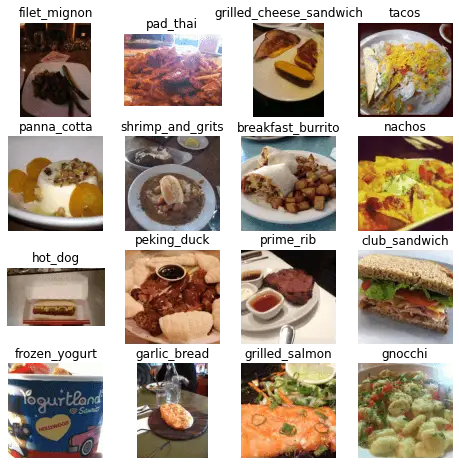
beignets

Let's explore the dataset a little bit more. The below code is a function that displays random images from the dataset along with their labels:

import random
import matplotlib.pyplot as plt

def show_image_grid(dataset, split, grid_size=(4,4)):
    # Select random images from the given split
    indices = random.sample(range(len(dataset[split])), grid_size[0]*grid_size[1])
    images = [dataset[split][i]["image"] for i in indices]
    labels = [dataset[split][i]["label"] for i in indices]
    
    # Display the images in a grid
    fig, axes = plt.subplots(nrows=grid_size[0], ncols=grid_size[1], figsize=(8,8))
    for i, ax in enumerate(axes.flat):
        ax.imshow(images[i])
        ax.axis('off')
        ax.set_title(ds["train"].features["label"].int2str(labels[i]))
    
    plt.show()

show_image_grid(ds, "train")

Output:

Preprocessing the Data

Now that we have successfully loaded our dataset, let's make the necessary preprocessing function and apply it to our dataset:

def transform(examples):
  # convert all images to RGB format, then preprocessing it
  # using our image processor
  inputs = image_processor([img.convert("RGB") for img in examples["image"]], return_tensors="pt")
  # we also shouldn't forget about the labels
  inputs["labels"] = examples["label"]
  return inputs

# use the with_transform() method to apply the transform to the dataset on the fly during training
dataset = ds.with_transform(transform)

Excellent. We're converting all the images to the RGB format, and then passing them to our image processor. We also set return_tensors="pt" to get PyTorch tensors so they'll be cast to our device. Let's see how the data looks like:

for item in dataset["train"]:
  print(item["pixel_values"].shape)
  print(item["labels"])
  break

Output:

torch.Size([3, 224, 224])
6

As expected, the image shape is (3, 224, 224) and the label is a scalar.

Let's get the dataset labels:

# extract the labels for our dataset
labels = ds["train"].features["label"].names
labels

Output:

['apple_pie',
 'baby_back_ribs',
 'baklava',
 'beef_carpaccio',
..<SNIPPED>..
 'takoyaki',
 'tiramisu',
 'tuna_tartare',
 'waffles']

A total of 101 labels. Let's make the collating function to stack our dataset into batches:

def collate_fn(batch):
  return {
      "pixel_values": torch.stack([x["pixel_values"] for x in batch]),
      "labels": torch.tensor([x["labels"] for x in batch]),
  }

Defining the Metrics

Since the Trainer API expects a compute_metrics() function. For this demo, I'll be using the accuracy and F1 score:

from evaluate import load
import numpy as np

# load the accuracy and f1 metrics from the evaluate module
accuracy = load("accuracy")
f1 = load("f1")

def compute_metrics(eval_pred):
  # compute the accuracy and f1 scores & return them
  accuracy_score = accuracy.compute(predictions=np.argmax(eval_pred.predictions, axis=1), references=eval_pred.label_ids)
  f1_score = f1.compute(predictions=np.argmax(eval_pred.predictions, axis=1), references=eval_pred.label_ids, average="macro")
  return {**accuracy_score, **f1_score}

I'm using the 🤗 evaluate module, but you're free to use any other module, such as sklearn. Nevertheless, the above code works. After calculating the scores, we're combining and finally return them.

Training the Model

To train our model, let's first re-initialize our model with the new labels. The original model had 1,000 classes in the output layer, so we have to set num_labels to the number of labels in our dataset, which is the length of our labels variable:

# load the ViT model
model = ViTForImageClassification.from_pretrained(
    model_name,
    num_labels=len(labels),
    id2label={str(i): c for i, c in enumerate(labels)},
    label2id={c: str(i) for i, c in enumerate(labels)},
    ignore_mismatched_sizes=True,
)

Next, defining the training arguments:

from transformers import TrainingArguments

training_args = TrainingArguments(
  output_dir="./vit-base-food", # output directory
  # output_dir="./vit-base-skin-cancer",
  per_device_train_batch_size=32, # batch size per device during training
  evaluation_strategy="steps",    # evaluation strategy to adopt during training
  num_train_epochs=3,             # total number of training epochs
  # fp16=True,                    # use mixed precision
  save_steps=1000,                # number of update steps before saving checkpoint
  eval_steps=1000,                # number of update steps before evaluating
  logging_steps=1000,             # number of update steps before logging
  # save_steps=50,
  # eval_steps=50,
  # logging_steps=50,
  save_total_limit=2,             # limit the total amount of checkpoints on disk
  remove_unused_columns=False,    # remove unused columns from the dataset
  push_to_hub=False,              # do not push the model to the hub
  report_to='tensorboard',        # report metrics to tensorboard
  load_best_model_at_end=True,    # load the best model at the end of training
)

Here we're setting some parameters. save_total_limit=2 means we only keep two model checkpoints in our disk, the best two.

We haven't set any optimizer parameters, so we're leaving everything to the default settings. For example, the initial learning rate of the default AdamW optimizer will be 5e-5. Therefore, there's definitely room for improvement here.

There are a lot of parameters in the TrainingArguments, I highly suggest you check this page to read more about the available parameters that fits your needs.

Let's make our trainer and start training:

from transformers import Trainer

trainer = Trainer(
    model=model,                        # the instantiated 🤗 Transformers model to be trained
    args=training_args,                 # training arguments, defined above
    data_collator=collate_fn,           # the data collator that will be used for batching
    compute_metrics=compute_metrics,    # the metrics function that will be used for evaluation
    train_dataset=dataset["train"],     # training dataset
    eval_dataset=dataset["validation"], # evaluation dataset
    tokenizer=image_processor,          # the processor that will be used for preprocessing the images
)

# start training
trainer.train()

Output:

***** Running training *****
  Num examples = 75750
  Num Epochs = 3
  Instantaneous batch size per device = 32
  Total train batch size (w. parallel, distributed & accumulation) = 32
  Gradient Accumulation steps = 1
  Total optimization steps = 7104
  Number of trainable parameters = 85876325
 [7104/7104 3:46:15, Epoch 3/3]
Step	Training Loss	Validation Loss	Accuracy	F1
1000	1.440300	    0.582373	    0.853149	0.852764
2000	0.703100	    0.453642	    0.878297	0.878230
3000	0.434700	    0.409464	    0.886455	0.886492
4000	0.310100	    0.394801	    0.889188	0.888990
5000	0.245100	    0.383308	    0.895168	0.895035
6000	0.115700	    0.379927	    0.896515	0.896743
7000	0.108100	    0.376985	    0.898059	0.898311

As you can see, the validation loss is still decreasing, and F1 and accuracy scores are increasing. I suggest you increase the number of epochs to get better results than mine.

You can run tensorboard on the vit-base-food/runs folder to see the loss and the metrics on the training and validation sets over time during training.

If you want to fine tune your model using a regular PyTorch loop, then you can have it in the Colab version.

If you have a test dataset, you can use the evaluate() method:

# trainer.evaluate(dataset["test"])

This will compute the metrics against the test dataset if you have one.

If you've canceled the training for some reason, then you have to run this to load the best-performing model:

# load the best model, change the checkpoint number to the best checkpoint
# if the last checkpoint is the best, then ignore this cell
best_checkpoint = 3000
# best_checkpoint = 150
model = ViTForImageClassification.from_pretrained(f"./vit-base-food/checkpoint-{best_checkpoint}").to(device)
# model = ViTForImageClassification.from_pretrained(f"./vit-base-skin-cancer/checkpoint-{best_checkpoint}").to(device)

If you didn't cancel the training, then the model will be the best one, so you won't have to execute the above.

Performing Inference

Let's use our get_prediction() function we defined earlier to perform inference on food images:

get_prediction(best_model, "https://images.pexels.com/photos/858496/pexels-photo-858496.jpeg?auto=compress&cs=tinysrgb&w=600&lazy=load")

sushi image

Output:

sushi

Excellent. Let's edit our get_prediction() function and add the ability to get the top most probable num_classes along with their probabilities:

def get_prediction_probs(model, url_or_path, num_classes=3):
    # load the image
    img = load_image(url_or_path)
    # preprocessing the image
    pixel_values = image_processor(img, return_tensors="pt")["pixel_values"].to(device)
    # perform inference
    output = model(pixel_values)
    # get the top k classes and probabilities
    probs, indices = torch.topk(output.logits.softmax(dim=1), k=num_classes)
    # get the class labels
    id2label = model.config.id2label
    classes = [id2label[idx.item()] for idx in indices[0]]
    # convert the probabilities to a list
    probs = probs.squeeze().tolist()
    # create a dictionary with the class names and probabilities
    results = dict(zip(classes, probs))
    return results

With the get_prediction_probs(), instead of performing the argmax() function, we use the torch.topk() method to get the top k classes. Let's use it:

# example 1
get_prediction_probs(best_model, "https://images.pexels.com/photos/406152/pexels-photo-406152.jpeg?auto=compress&cs=tinysrgb&w=600")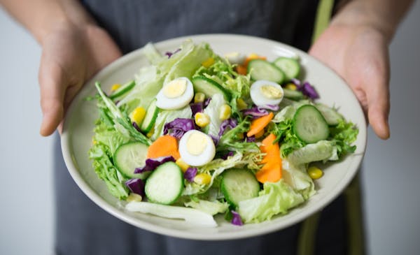

Output:

{'greek_salad': 0.9658474326133728,
 'caesar_salad': 0.019217027351260185,
 'beet_salad': 0.008294313214719296}

# example 2
get_prediction_probs(best_model, "https://images.pexels.com/photos/920220/pexels-photo-920220.jpeg?auto=compress&cs=tinysrgb&w=600")

Output:

{'grilled_cheese_sandwich': 0.9855711460113525,
 'waffles': 0.0030371786560863256,
 'club_sandwich': 0.0017941497499123216}

# example 3
get_prediction_probs(best_model, "https://images.pexels.com/photos/3338681/pexels-photo-3338681.jpeg?auto=compress&cs=tinysrgb&w=600")

Output:

{'donuts': 0.9919546246528625,
 'cup_cakes': 0.0018467127811163664,
 'beignets': 0.0009919782169163227}

Here is a final example, where we set num_classes to 10 for instance:

# example 4
get_prediction_probs(best_model, "https://images.pexels.com/photos/806457/pexels-photo-806457.jpeg?auto=compress&cs=tinysrgb&w=600", num_classes=10)

Output:

{'deviled_eggs': 0.9846165180206299,
 'caprese_salad': 0.0012617064639925957,
 'ravioli': 0.001060450915247202,
 'beet_salad': 0.0008713295101188123,
 'scallops': 0.0005976424436084926,
 'gnocchi': 0.0005376451299525797,
 'fried_calamari': 0.0005195785779505968,
 'caesar_salad': 0.0003912363899871707,
 'samosa': 0.0003842405858449638,
 'dumplings': 0.00036707069375552237}

Conclusion

Fine-tuning Vision Transformer (ViT) on image classification using 🤗 Transformers is a powerful technique that can significantly improve the performance of computer vision models. The use of ViT enables the efficient processing of large images with high resolution, while the 🤗 Transformers library provides a user-friendly and efficient platform for training and evaluation.

Through this tutorial, we have learned how to fine-tune a pre-trained ViT model for image classification tasks, including how to preprocess the data, create a custom dataset, and fine-tune the model using the Trainer API. By following these steps and experimenting with different hyperparameters (check this link), it is possible to achieve state-of-the-art results on various image classification datasets.

We hope this tutorial has provided a useful introduction to this exciting area of computer vision and encouraged you to further explore the possibilities of ViT and 🤗 Transformers for image classification tasks.

You can get the complete code here, or Colab here.

Here are some related tutorials:

Happy learning ♥

Ready for more? Dive deeper into coding with our AI-powered Code Explainer. Don't miss it!

View Full Code Assist My Coding

Sharing is caring!

Read Also

How to Perform Image Segmentation using Transformers in Python

Comment panel

Got a coding query or need some guidance before you comment? Check out this Python Code Assistant for expert advice and handy tips. It's like having a coding tutor right in your fingertips!