How to Perform YOLO Object Detection using OpenCV in Python

Kickstart your coding journey with our Python Code Assistant. An AI-powered assistant that's always ready to help. Don't miss out!

Object detection is a task in computer vision and image processing that deals with detecting objects in images or videos. It is used in a wide variety of real-world applications, including video surveillance, self-driving cars, object tracking, etc.

For instance, for a car to be truly autonomous, it must identify and keep track of surrounding objects (such as cars, pedestrians, and traffic lights). One of the primary sources of information is the camera, which uses object detection. On top of that, the detection should be in real-time, which requires a relatively fast way so that the car can safely navigate the street.

This tutorial will teach you how to perform object detection using the YOLOv3 technique with OpenCV or PyTorch in Python. After that, we will also dive into the current state-of-the-art, which is an improved version of YOLO, that is YOLOv8.

Related: How to Perform Image Segmentation using Transformers in Python.

YOLO (You Only Look Once) is a real-time object detection algorithm that is a single deep convolutional neural network that splits the input image into a set of grid cells, so unlike image classification or face detection, each grid cell in the YOLO algorithm will have an associated vector in the output that tells us:

• If an object exists in that grid cell.
• The class of that object (i.e., label).
• The predicted bounding box for that object (location).

There are other approaches, such as Fast R-CNN, Faster R-CNN, which use window slides over the image, making it requires thousands of predictions on a single image (on each window); as you may guess, this makes YOLOv8 more than1000x faster than R-CNN and even over 100x faster than Fast R-CNN.

YOLO version 8 is the latest version of YOLO, which uses a lot of tricks to improve accuracy and increase performance. Check the full details in the Ultralytics YOLOv8 docs.

Here is the table of contents:

• Using YOLOv3
  • Getting Started
  • Preparing the Image
  • Making Predictions
  • Drawing Detected Objects
  • Non-Maximal Suppression
    • What is IoU
  • PyTorch Code
• Updated: Using YOLOv8
  • Loading the Model
  • Making Predictions
  • Drawing Detected Objects
• Conclusion

Using YOLOv3

Getting Started

Before we dive into the code, let's install the required libraries for this tutorial (If you want to use PyTorch code, head to this page for installation):

pip3 install opencv-python numpy matplotlib

It is pretty challenging to build YOLOv3 whole system (the model and the techniques used) from scratch. Open-source libraries such as Darknet or OpenCV already made that for you or even ordinary people who built third-party projects for YOLOv3 (For example, this link is a TensorFlow implementation)

Importing required modules:

import cv2
import numpy as np

import time
import sys
import os

Let's define some variables and parameters that we are going to need:

CONFIDENCE = 0.5
SCORE_THRESHOLD = 0.5
IOU_THRESHOLD = 0.5

# the neural network configuration
config_path = "cfg/yolov3.cfg"
# the YOLO net weights file
weights_path = "weights/yolov3.weights"
# weights_path = "weights/yolov3-tiny.weights"

# loading all the class labels (objects)
labels = open("data/coco.names").read().strip().split("\n")
# generating colors for each object for later plotting
colors = np.random.randint(0, 255, size=(len(LABELS), 3), dtype="uint8")

We initialized our parameters; we will talk about them later on, config_path and weights_path represents the model configuration (of yolov3) and the corresponding pre-trained model weights, respectively. labels is the list of all class labels for different objects to detect. We will draw each object class with a unique color. That's why we generated random colors.

Please refer to this repository for the required files, and since the weights file is so huge (about 240MB), it isn't in the repository. Please download it here.

The below code loads the model:

# load the YOLO network
net = cv2.dnn.readNetFromDarknet(config_path, weights_path)

Preparing the Image

Let's load an example image (the image among others in the GitHub repository):

path_name = "images/street.jpg"
image = cv2.imread(path_name)
file_name = os.path.basename(path_name)
filename, ext = file_name.split(".")

Next, we need to normalize, scale, and reshape this image to be suitable as an input to the neural network:

h, w = image.shape[:2]
# create 4D blob
blob = cv2.dnn.blobFromImage(image, 1/255.0, (416, 416), swapRB=True, crop=False)

This will normalize pixel values to range from 0 to 1, resize the image to (416, 416), and reshape it. Let's see:

print("image.shape:", image.shape)
print("blob.shape:", blob.shape)

Output:

image.shape: (1200, 1800, 3)
blob.shape: (1, 3, 416, 416)

Related: Satellite Image Classification using TensorFlow in Python.

Making Predictions

Now let's feed this image into the neural network to get the output predictions:

# sets the blob as the input of the network
net.setInput(blob)
# get all the layer names
ln = net.getLayerNames()
try:
    ln = [ln[i[0] - 1] for i in net.getUnconnectedOutLayers()]
except IndexError:
    # in case getUnconnectedOutLayers() returns 1D array when CUDA isn't available
    ln = [ln[i - 1] for i in net.getUnconnectedOutLayers()]
# feed forward (inference) and get the network output
# measure how much it took in seconds
start = time.perf_counter()
layer_outputs = net.forward(ln)
time_took = time.perf_counter() - start
print(f"Time took: {time_took:.2f}s")

This will extract the neural network output and print the total time taken in inference:

Time took: 1.54s

Now you're maybe wondering why it isn't that fast? 1.5 seconds is pretty slow? We're using our CPU only for inference, which is not ideal for real-world problems. That's why we'll jump into PyTorch later in this tutorial. On the other hand, 1.5 seconds is relatively good compared to other techniques such as R-CNN.

You can also use the tiny version of YOLOv3, which is much faster but less accurate. You can download it here.

Now we need to iterate over the neural network outputs and discard any object with confidence less than the CONFIDENCE parameter we specified earlier (i.e 0.5 or 50%).

font_scale = 1
thickness = 1
boxes, confidences, class_ids = [], [], []
# loop over each of the layer outputs
for output in layer_outputs:
    # loop over each of the object detections
    for detection in output:
        # extract the class id (label) and confidence (as a probability) of
        # the current object detection
        scores = detection[5:]
        class_id = np.argmax(scores)
        confidence = scores[class_id]
        # discard out weak predictions by ensuring the detected
        # probability is greater than the minimum probability
        if confidence > CONFIDENCE:
            # scale the bounding box coordinates back relative to the
            # size of the image, keeping in mind that YOLO actually
            # returns the center (x, y)-coordinates of the bounding
            # box followed by the boxes' width and height
            box = detection[:4] * np.array([w, h, w, h])
            (centerX, centerY, width, height) = box.astype("int")
            # use the center (x, y)-coordinates to derive the top and
            # and left corner of the bounding box
            x = int(centerX - (width / 2))
            y = int(centerY - (height / 2))
            # update our list of bounding box coordinates, confidences,
            # and class IDs
            boxes.append([x, y, int(width), int(height)])
            confidences.append(float(confidence))
            class_ids.append(class_id)

This will loop over all the predictions and only save the objects with high confidence. Let's see what the detection vector represents:

print(detection.shape)

Output:

(85,)

On each object prediction, there is a vector of 85. The first four values represent the location of the object, (x, y) coordinates for the centering point and the width and the height of the bounding box, and the remaining numbers correspond to the object labels since this is the COCO dataset. It has 80 class labels.

For instance, if the object detected is a person, the first value in the 80 length vector should be 1 and all the remaining values should be 0, the 2nd number for bicycle, 3rd for car, all the way to the 80th object. We're using the np.argmax() function to get the class id, as it returns the index of the maximum value from that 80 length vector.

Drawing Detected Objects

Now we have all we need, let's draw the object rectangles and labels and see the result:

# loop over the indexes we are keeping
for i in range(len(boxes)):
    # extract the bounding box coordinates
    x, y = boxes[i][0], boxes[i][1]
    w, h = boxes[i][2], boxes[i][3]
    # draw a bounding box rectangle and label on the image
    color = [int(c) for c in colors[class_ids[i]]]
    cv2.rectangle(image, (x, y), (x + w, y + h), color=color, thickness=thickness)
    text = f"{labels[class_ids[i]]}: {confidences[i]:.2f}"
    # calculate text width & height to draw the transparent boxes as background of the text
    (text_width, text_height) = cv2.getTextSize(text, cv2.FONT_HERSHEY_SIMPLEX, fontScale=font_scale, thickness=thickness)[0]
    text_offset_x = x
    text_offset_y = y - 5
    box_coords = ((text_offset_x, text_offset_y), (text_offset_x + text_width + 2, text_offset_y - text_height))
    overlay = image.copy()
    cv2.rectangle(overlay, box_coords[0], box_coords[1], color=color, thickness=cv2.FILLED)
    # add opacity (transparency to the box)
    image = cv2.addWeighted(overlay, 0.6, image, 0.4, 0)
    # now put the text (label: confidence %)
    cv2.putText(image, text, (x, y - 5), cv2.FONT_HERSHEY_SIMPLEX,
        fontScale=font_scale, color=(0, 0, 0), thickness=thickness)

Let's write the image:

cv2.imwrite(filename + "_yolo3." + ext, image)

A new image will appear in the current directory that labels each object detected with confidence. However, look at this part of the image:

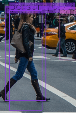
You guessed it, two bounding boxes for a single object; this is a problem, isn't it? Well, the creators of YOLO used a technique called Non-maximal Suppression to eliminate this.

Non-Maximal Suppression

Non-Maximal Suppression is a technique that suppresses overlapping bounding boxes that do not have the maximum probability for object detection. It is mainly achieved in two phases:

• It selects the bounding box with the highest confidence (i.e., probability).
• It then compares all other bounding boxes with this selected bounding box and eliminates the ones that have a high IoU.

What is IoU

IoU (Intersection over Union) is a technique used in Non-Maximal Suppression to compare how close two different bounding boxes are. It is demonstrated in the following figure:

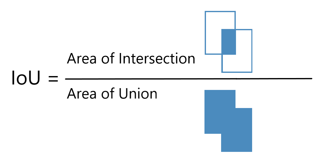
The higher the IoU, the closer the bounding boxes are. An IoU of 1 means that the two bounding boxes are identical, while an IoU of 0 means that they're not even intersected.

As a result, we will be using an IoU threshold value of 0.5 (which we initialized at the beginning of this tutorial), which means that we eliminate any bounding box below this value compared to that maximal probability bounding box.

The SCORE_THRESHOLD will eliminate any bounding box that has the confidence below that value:

# perform the non maximum suppression given the scores defined before
idxs = cv2.dnn.NMSBoxes(boxes, confidences, SCORE_THRESHOLD, IOU_THRESHOLD)

Now let's draw the boxes again:

# ensure at least one detection exists
if len(idxs) > 0:
    # loop over the indexes we are keeping
    for i in idxs.flatten():
        # extract the bounding box coordinates
        x, y = boxes[i][0], boxes[i][1]
        w, h = boxes[i][2], boxes[i][3]
        # draw a bounding box rectangle and label on the image
        color = [int(c) for c in colors[class_ids[i]]]
        cv2.rectangle(image, (x, y), (x + w, y + h), color=color, thickness=thickness)
        text = f"{labels[class_ids[i]]}: {confidences[i]:.2f}"
        # calculate text width & height to draw the transparent boxes as background of the text
        (text_width, text_height) = cv2.getTextSize(text, cv2.FONT_HERSHEY_SIMPLEX, fontScale=font_scale, thickness=thickness)[0]
        text_offset_x = x
        text_offset_y = y - 5
        box_coords = ((text_offset_x, text_offset_y), (text_offset_x + text_width + 2, text_offset_y - text_height))
        overlay = image.copy()
        cv2.rectangle(overlay, box_coords[0], box_coords[1], color=color, thickness=cv2.FILLED)
        # add opacity (transparency to the box)
        image = cv2.addWeighted(overlay, 0.6, image, 0.4, 0)
        # now put the text (label: confidence %)
        cv2.putText(image, text, (x, y - 5), cv2.FONT_HERSHEY_SIMPLEX,
            fontScale=font_scale, color=(0, 0, 0), thickness=thickness)

You can use cv2.imshow("image", image) to show the image, but we are just going to save it to disk:

cv2.imwrite(filename + "_yolo3." + ext, image)

Check this out:

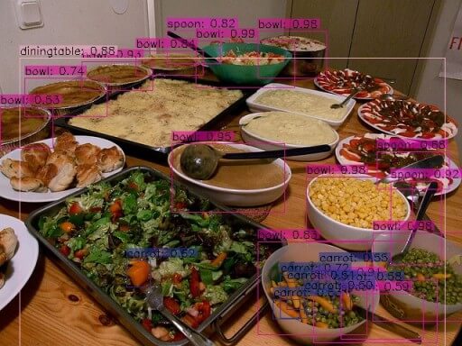
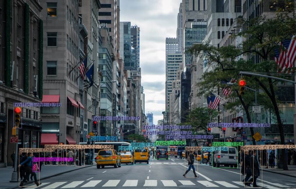Here is another sample image:

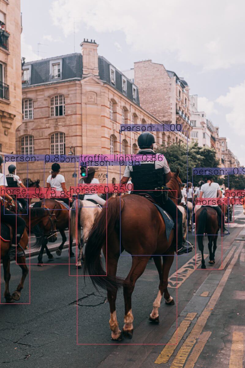
Or this:

Awesome! Use your own images and tweak those parameters and see which works best!

Also, if the image got a high resolution, make sure you increase the font_scale parameter to see the bounding boxes and their corresponding labels.

PyTorch Code

As mentioned earlier, if you want to use a GPU (which is much faster than a CPU) for inference, then you can use the PyTorch library, which supports CUDA computing. Here is the code for that (get darknet.py and utils.py from the repository):

import cv2
import matplotlib.pyplot as plt
from utils import *
from darknet import Darknet

# Set the NMS Threshold
nms_threshold = 0.6
# Set the IoU threshold
iou_threshold = 0.4
cfg_file = "cfg/yolov3.cfg"
weight_file = "weights/yolov3.weights"
namesfile = "data/coco.names"
m = Darknet(cfg_file)
m.load_weights(weight_file)
class_names = load_class_names(namesfile)
# m.print_network()
original_image = cv2.imread("images/city_scene.jpg")
original_image = cv2.cvtColor(original_image, cv2.COLOR_BGR2RGB)
img = cv2.resize(original_image, (m.width, m.height))
# detect the objects
boxes = detect_objects(m, img, iou_threshold, nms_threshold)
# plot the image with the bounding boxes and corresponding object class labels
plot_boxes(original_image, boxes, class_names, plot_labels=True)

Note: The above code requires darknet.py and utils.py files in the current directory. Also, PyTorch must be installed (GPU accelerated is suggested).

Learn also: Real-time Object Tracking with OpenCV and YOLOv8 in Python.

Updated: Using YOLOv8

In the previous section, we saw how to use YOLO version 3 but the YOLO model has gone through several iterations since then, and now we have YOLO version 8. In this section, we will see how to use YOLO version 8 for object detection with OpenCV.

From version 3 of YOLO to version 8, a lot of things have changed and improved. With each iteration, the model has become more accurate and faster at the same time. And of course, now it's a lot easier to use YOLO for object detection.

For instance, Non-maximal Suppression (NMS) is now built into the model. So, we don't have to worry about it anymore. 

To get started, make sure to install ultralytics:

$ pip install ultralytics

Create a new file yolov8_opencv.py and import the following:

import numpy as np
import os
import cv2
import time
from ultralytics import YOLO

We will use the YOLO class from the ultralytics library to load the YOLOv8 model. 

Loading the Model

Now let's define some parameters and load our model:

# define some parameters
CONFIDENCE = 0.5
font_scale = 1
thickness = 1

# loading the YOLOv8 model with the default weight file
model = YOLO("yolov8n.pt")

# loading all the class labels (objects)
labels = open("data/coco.names").read().strip().split("\n")

# generating colors for each object for later plotting
colors = np.random.randint(0, 255, size=(len(labels), 3), dtype="uint8")

There are 5 different models available for YOLOv8: yolov8n, yolov8s, yolov8m, yolov8l, and yolov8x. From the fastest and light-weight (less accurate) to the more accurate one. You can find more information about them here.

We will use the yolov8n model for this tutorial. The model will be downloaded automatically when you run the script for the first time.

Related: Real-time Object Tracking with OpenCV and YOLOv8 in Python.

Making Predictions

Now let's load the image and get the predictions:

path_name = "images/dog.jpg"
image = cv2.imread(path_name)
file_name = os.path.basename(path_name) # "dog.jpg"
filename, ext = file_name.split(".") # "dog", "jpg"

# measure how much it took in seconds
start = time.perf_counter()
# run inference on the image 
# see: https://docs.ultralytics.com/modes/predict/#arguments for full list of arguments
results = model.predict(image, conf=CONFIDENCE)[0]
time_took = time.perf_counter() - start
print(f"Time took: {time_took:.2f}s")
print(results.boxes.data)

Here we are using the same code as before to load the image. Then we are using the predict() method of the YOLO class to get the predictions.

The predict() method takes a lot of arguments. You can find the full list of arguments here. In the code above, we are passing the image and the confidence threshold to the predict() method so that it only returns the predictions with a confidence score greater than 0.5.

The results variable will contain the bounding boxes, confidence scores, and class IDs for each object detected in the image.

We can use the results.boxes.data to get the output from the model:

0: 480x640 1 bicycle, 1 car, 1 dog, 43.0ms
Speed: 3.5ms preprocess, 43.0ms inference, 0.8ms postprocess per image at shape (1, 3, 640, 640)
Time took: 0.14s
tensor([[1.3113e+02, 2.1990e+02, 3.0930e+02, 5.4196e+02, 9.0973e-01, 1.6000e+01],
        [1.3056e+02, 1.3924e+02, 5.6825e+02, 4.2083e+02, 8.8791e-01, 1.0000e+00],
        [4.6761e+02, 7.4896e+01, 6.9218e+02, 1.7169e+02, 5.4889e-01, 2.0000e+00]])

As you can see, the output is a tensor with 6 columns. The first 4 columns are the bounding box coordinates, the 5th column is the confidence score, and the last column is the class ID.

The total time taken to run the whole process is 0.14 seconds.

Drawing Detected Objects

So, now we can loop over the results and draw the bounding boxes on the image:

# loop over the detections
for data in results.boxes.data.tolist():
    # get the bounding box coordinates, confidence, and class id 
    xmin, ymin, xmax, ymax, confidence, class_id = data
    # converting the coordinates and the class id to integers
    xmin = int(xmin)
    ymin = int(ymin)
    xmax = int(xmax)
    ymax = int(ymax)
    class_id = int(class_id)

    # draw a bounding box rectangle and label on the image
    color = [int(c) for c in colors[class_id]]
    cv2.rectangle(image, (xmin, ymin), (xmax, ymax), color=color, thickness=thickness)
    text = f"{labels[class_id]}: {confidence:.2f}"
    # calculate text width & height to draw the transparent boxes as background of the text
    (text_width, text_height) = cv2.getTextSize(text, cv2.FONT_HERSHEY_SIMPLEX, fontScale=font_scale, thickness=thickness)[0]
    text_offset_x = xmin
    text_offset_y = ymin - 5
    box_coords = ((text_offset_x, text_offset_y), (text_offset_x + text_width + 2, text_offset_y - text_height))
    overlay = image.copy()
    cv2.rectangle(overlay, box_coords[0], box_coords[1], color=color, thickness=cv2.FILLED)
    # add opacity (transparency to the box)
    image = cv2.addWeighted(overlay, 0.6, image, 0.4, 0)
    # now put the text (label: confidence %)
    cv2.putText(image, text, (xmin, ymin - 5), cv2.FONT_HERSHEY_SIMPLEX,
        fontScale=font_scale, color=(0, 0, 0), thickness=thickness)

# display output image
cv2.imshow("Image", image)
cv2.waitKey(0)
# save output image to disk
cv2.imwrite(filename + "_yolo8." + ext, image)

The code above is the same as before. The only difference is that we are looping over the results.boxes.data.tolist() and extracting the bounding box coordinates, confidence score, and class ID for each object detected in the image.

Then, we draw the bounding box rectangle and label it on the image.

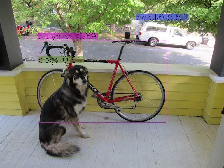
After you run the code, you should see a new image created in the current directory with the bounding boxes and labels drawn on it:

Conclusion

Amazing! In this tutorial, you learned how to perform object detection with OpenCV. We first used the previous YOLOv3 version and then dived into the current state-of-the-art YOLOv8 model.

I have prepared a code for you to use your live camera for real-time YOLOv8 object detection; check it out here. Also, if you want to read a video file and make object detection on it, this code can help you. Here is an example output video:

Here are some useful resources for further reading:

• Ultralytics YOLOv8 Docs
• YOLOv3: Real-time Object Detection

You can get the complete code for everything here.

Learn also: Skin Cancer Detection using TensorFlow in Python.

Happy Learning ♥

Take the stress out of learning Python. Meet our Python Code Assistant – your new coding buddy. Give it a whirl!

Read Also

Real-time Object Tracking with OpenCV and YOLOv8 in Python

Learn how to perform real-time object tracking with the DeepSORT algorithm and YOLOv8 using the OpenCV library in Python.

How to Use Transfer Learning for Image Classification using TensorFlow in Python

Learn what is transfer learning and how to use pre trained MobileNet model for better performance to classify flowers using TensorFlow in Python.

Satellite Image Classification using TensorFlow in Python

Learn how to fine-tune the current state-of-the-art EffecientNet V2 model to perform image classification on satellite data (EuroSAT) using TensorFlow in Python.

Comment panel