Welcome! Meet our Python Code Assistant, your new coding buddy. Why wait? Start exploring now!
Introduction
Since model performance may be considerably enhanced by fine-tuning their hyperparameters, tuning them involves identifying optimum parameters that will provide more outstanding performance than the model's default hyperparameters. We can use several techniques for hyperparameter tuning. One of them is the dropout.
In this tutorial, we will present dropout regularization for neural networks. We first explore the background and motivation for adopting dropout, followed by a description of how dropout works theoretically and how to implement it in the Pytorch library in Python.
We will also see a plot of the loss on the testing set through time on the neural network with and without dropout.
Table of content:
- Introduction
- Setting Everything Up
- Training A Neural Network without Dropout
- Common Problems in Neural Networks
- Introducing Dropout
- Training A Neural Network with Dropout
- Conclusion
Setting Everything Up
For demonstration, we'll be using the MNIST dataset that is available in the torchvision library. Let's install all the dependencies of this tutorial:
$ pip install matplotlib==3.4.3 numpy==1.21.5 torch==1.10.1 torchvisionIf you're on Colab, you don't have to install anything, as everything comes pre-installed. Importing the necessary libraries:
import torch
import torchvision
import torchvision.transforms as transforms
import matplotlib.pyplot as plt
import numpy as np
Let's make sure we train using GPU if CUDA is available:
# defining our device, 'cuda:0' if CUDA is available, 'cpu' otherwise
device = torch.device('cuda:0' if torch.cuda.is_available() else 'cpu')
device
device(type='cuda', index=0)Let's make the transform pipeline for our MNIST dataset:
# make the transform pipeline, converting to tensor and normalizing
transform = transforms.Compose([
  transforms.ToTensor(),
  transforms.Normalize((0.5, 0.5, 0.5), (0.5, 0.5, 0.5))
])
# the batch size during training
batch_size = 64
Next, loading the training dataset:
train_dataset = torchvision.datasets.CIFAR10(root="./data", train=True,
                                             download=True, transform=transform)
train_loader = torch.utils.data.DataLoader(train_dataset, batch_size=batch_size,
                                           shuffle=True, num_workers=2)
Downloading https://www.cs.toronto.edu/~kriz/cifar-10-python.tar.gz to ./data/cifar-10-python.tar.gz
170499072/? [00:06<00:00, 29640614.08it/s]
Extracting ./data/cifar-10-python.tar.gz to ./dataWe pass True to train to indicate the training dataset, and we also set download to True to download the dataset into the specified data folder. After that, we make our DataLoader, pass the batch_size, and set shuffle to True.
Similarly, for the test set:
test_dataset = torchvision.datasets.CIFAR10(root="./data", train=False,
                                             download=True, transform=transform)
test_loader = torch.utils.data.DataLoader(test_dataset, batch_size=batch_size,
                                           shuffle=False, num_workers=2)
Files already downloaded and verifiedThis time we set train to False to get the testing set.
Below are the available classes in the MNIST dataset:
# the MNIST classes
classes = ('plane', 'car', 'bird', 'cat',
           'deer', 'dog', 'frog', 'horse', 'ship', 'truck')
Training A Neural Network without Dropout
Now that we have the dataset ready for training, let's make a neural network without dropout:
import torch.nn as nn
import torch.nn.functional as F

class Net(nn.Module):
    def __init__(self):
        super().__init__()
        self.conv1 = nn.Conv2d(3, 6, 5)
        self.pool = nn.MaxPool2d(2, 2)
        self.conv2 = nn.Conv2d(6, 16, 5)
        self.fc1 = nn.Linear(16 * 5 * 5, 120)
        self.fc2 = nn.Linear(120, 84)
        self.fc3 = nn.Linear(84, 10)

    def forward(self, x):
        x = self.pool(F.relu(self.conv1(x)))
        x = self.pool(F.relu(self.conv2(x)))
        x = torch.flatten(x, 1) # flatten all dimensions except batch
        x = F.relu(self.fc1(x))
        x = F.relu(self.fc2(x))
        x = self.fc3(x)
        return x

net = Net()
# switch to GPU if available
net.to(device)
Initializing the cross-entropy loss and the SGD optimizer:
import torch.optim as optim

# defining the loss and the optimizer
criterion = nn.CrossEntropyLoss()
optimizer = optim.SGD(net.parameters(), lr=0.001, momentum=0.9)
Next, let's make a function that accepts the neural network, the loss, and the data loader to calculate the overall loss:
def get_test_loss(net, criterion, data_loader):
  """A simple function that iterates over `data_loader` to calculate the overall loss"""
  testing_loss = []
  with torch.no_grad():
    for data in data_loader:
      inputs, labels = data
      # get the data to GPU (if available)
      inputs, labels = inputs.to(device), labels.to(device)
      outputs = net(inputs)
      # calculate the loss for this batch
      loss = criterion(outputs, labels)
      # add the loss of this batch to the list
      testing_loss.append(loss.item())
  # calculate the average loss
  return sum(testing_loss) / len(testing_loss)
We'll be needing this function during training. Let's start training now:
training_loss, testing_loss = [], []
running_loss = []
i = 0
for epoch in range(150): # 150 epochs
  for data in train_loader:
    inputs, labels = data
    # get the data to GPU (if available)
    inputs, labels = inputs.to(device), labels.to(device)
    optimizer.zero_grad()
    # forward pass
    outputs = net(inputs)
    # backward pass
    loss = criterion(outputs, labels)
    loss.backward()
    # update gradients
    optimizer.step()
    running_loss.append(loss.item())
    i += 1
    if i % 1000 == 0:
      avg_train_loss = sum(running_loss) / len(running_loss)
      avg_test_loss = get_test_loss(net, criterion, test_loader)
      # clear the list
      running_loss.clear()
      # for logging & plotting later
      training_loss.append(avg_train_loss)
      testing_loss.append(avg_test_loss)
      print(f"[{epoch:2d}] [it={i:5d}] Train Loss: {avg_train_loss:.3f}, Test Loss: {avg_test_loss:.3f}")

print("Done training.")
Output:
[ 1] [it= 1000] Train Loss: 2.273, Test Loss: 2.118
[10] [it= 8000] Train Loss: 1.312, Test Loss: 1.326
[20] [it=16000] Train Loss: 1.031, Test Loss: 1.120
[30] [it=24000] Train Loss: 0.854, Test Loss: 1.043
[40] [it=32000] Train Loss: 0.718, Test Loss: 1.051
[51] [it=40000] Train Loss: 0.604, Test Loss: 1.085
[60] [it=47000] Train Loss: 0.521, Test Loss: 1.178
[70] [it=55000] Train Loss: 0.425, Test Loss: 1.370
[80] [it=63000] Train Loss: 0.348, Test Loss: 1.518
[93] [it=73000] Train Loss: 0.268, Test Loss: 1.859
[99] [it=78000] Train Loss: 0.248, Test Loss: 2.036
[109] [it=86000] Train Loss: 0.200, Test Loss: 2.351
[120] [it=94000] Train Loss: 0.161, Test Loss: 2.610
[130] [it=102000] Train Loss: 0.142, Test Loss: 2.976
[140] [it=110000] Train Loss: 0.117, Test Loss: 3.319
[149] [it=117000] Train Loss: 0.095, Test Loss: 3.593
Done training.
Common Problems in Neural Networks
Overfitting
Deep neural networks include several non-linear hidden layers, making them highly expressive models capable of learning complex correlations between inputs and outputs. However, with minimal training data, many of these complex associations will result from sampling noise; thus, they will exist in the training set but not in the actual test data, even if they are derived from the same distribution. Fitting all feasible alternative neural networks on the same dataset and averaging the predictions from each model is one method for reducing overfitting.
It is impossible, but it may be approximated by utilizing a small group of distinct models known as an ensemble.
Bagging
Individually trained nets are costly with massive neural networks. Combining many models is most useful when the individual models are distinct from one another, and neural net models should be specific by having various designs or being trained on separate data. Training many designs is difficult because determining ideal hyperparameters for each architecture is a demanding undertaking, and training each huge network demands a significant amount of computing.
Furthermore, extensive networks often need a considerable quantity of training data, and there may not be enough data to train separate networks on different subsets of the data. So, even with the ensemble approximation, there is a difficulty in that it needs various models to be fit and stored, which may be challenging if the models are huge and take days or weeks to train and tune.
During training, the network's capacity is reduced when the outputs of a layer under dropout are randomly subsampled. Consequently, dropouts may need a more extensive network.
Introducing Dropout
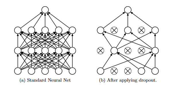
When training neural networks with dropout, specific layer outputs are disregarded or dropped out at random. This has the effect of having the layer having a different number of nodes and connectedness to the preceding layer.
Each update to a layer during training is made with a distinct view of the configured layer. Dropout makes the training process noisy, causing nodes within a layer to take on more or less responsibility for the inputs on a probabilistic basis.
On the training data, neurons learn to correct errors committed by their peers, a process known as co-adaptation. Consequently, the network's ability to fit the training data improves dramatically. Because the co-adaptations are tailored to the training data's particularities, they won't generalize to the test data; therefore, it becomes more volatile.
Nitish Srivastava, Ilya Sutskever, Geoffrey Hinton, Alex Krizhevsky, and Ruslan Salakhutdinov were the first to propose dropout to minimize the effects of neural co-adaptation.
 Source: the paper.
Randomly Dropping Nodes
Dropout is a technique that addresses both issues mentioned above in neural networks. It avoids overfitting and enables the effective approximation combining of an indefinitely large number of unique neural network topologies.
Dropout refers to removing units (both hidden and apparent) from a neural network. Dropping a unit out implies temporarily removing it from the network, including all of its incoming and outgoing connections. Dropout mimics a sparse activation from a given layer, which pushes the network to learn a sparse representation as a side-effect. It might be employed instead of activity regularization to encourage sparse representations in autoencoder models.
The Dropout Rate
Dropout adds a new hyperparameter: the likelihood of keeping a unit p. This hyperparameter controls the degree of Dropout.
There is no dropout when p = 1, and low p values indicate that there are a lot of dropouts. For concealed units, typical p values range from 0.5 to 0.8.
The kind of input influences the choice of input layers. A typical value for real-valued inputs (image patches or audio frames) is 0.8.
The choice of p for hidden layers is linked to the number of hidden units n. Smaller p demands large n, which slows down training and leads to underfitting.
When p is large, there may not be enough Dropout to avoid overfitting. In a particular layer, Units will have a 70% chance of remaining active and a 30% risk of being dropped if the retention probability is 0.7% in that layer.
Please note that PyTorch and other deep learning frameworks use a dropout rate instead of a keep rate p, a 70% keep rate means a 30% dropout rate, and so on.
Practical Hints for Dropout Regularization
- Dropout Rate: The dropout hyperparameter's default meaning is the likelihood of training a particular node in a layer, where 1.0 implies no dropout and 0.0 denotes no layer outputs.
- Use of a Broader Network: Larger networks (with more layers or nodes) are more prone to overfitting the training data. When utilizing dropout regularization, bigger networks may be used less danger of overfitting.
- Grided Search Parameters: Test various rates methodically rather than assuming a reasonable dropout rate for your network. Test different rates methodically. You can test values ranging from 1.0 to 0.1 in 0.1 increments.
- Use a Weight Restriction: Network weights will grow due to the probabilistic elimination of layer activations. A significant weight size might indicate an unstable network. To counteract this effect, a weight restriction may be applied to compel the norm (magnitude) of all weights in a layer to be less than a particular value.
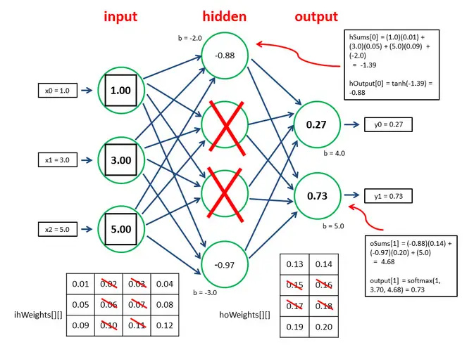
Dropout on Inference
When training, dropouts are solely used to increase the network's ability to withstand changes in the training dataset. During the test, you'll likely want to use the whole network.
Notably, dropout is not used with test data or during production inference. The result is that you will have more connections and activations in your neuron during inference than during training.
The neurons in the subsequent layer would thus be overexcited if you utilize a 50% dropout rate during training and remove two out of every four neurons in a layer. Thus, the values produced by these neurons will be 50% larger than necessary. Retention probability (1 – dropout rate) is used to scale down the weights of overactivated neurons during test and inference time. The figure below, created by Datascience Stackexchange member Dmytro Prylipko, beautifully depicts how this works:
Examples Using Dropout
First introduced by Geoffrey Hinton and colleagues in their 2012 paper titled Improving neural networks by preventing co-adaptation of feature detectors, dropout has been applied to a wide range of problem types, including photo classification (CIFAR-10), handwritten digit recognition (MNIST), and speech recognition (TIMIT).
This paper can deduce some interesting facts about dropout applications on the MNIST dataset.
- MNIST, a well-used benchmark for machine learning systems, was utilized to examine the efficacy of dropout. 60,000 28x28 training photos of handwritten digits and 10,000 test images are included in the database.
- Enhancing the training data with transformed images or wiring spatial transformation knowledge into a convolutional neural network, or employing generative pre-training to extract useful features from the training images without using the labels can significantly improve performance on the test set.
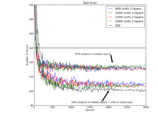
- The best-reported score for a regular feedforward neural network is 160 errors on the test set without applying any of these strategies.
By taking out a random 20 percent of the pixels, this may be lowered to roughly 130 errors and even further to about 110 errors by applying distinct L2 constraints to the incoming weights of each concealed unit. - Dropout was paired with generative pre-training, but only a tiny learning rate was utilized. No weight restrictions were applied to prevent losing the feature detectors identified by the pre-training. After being fine-tuned using ordinary back-propagation, the publicly accessible, pre-trained deep belief net made 118 errors and a total of 92 errors after being fine-tuned using 50 percent dropout of the hidden units.
- The below figure presents neural networks trained using backpropagation using 50% dropout for all hidden layers on the MNIST test set, and dropout is 20% on the lowest set of lines. The best previously reported result using backpropagation without pre-training, weight-sharing, or training session upgrades is displayed on the horizontal line.
 When dropout was introduced in a 2014 journal publication entitled Dropout: A Simple Way to Prevent Neural Networks from Overfitting, it was tried on a wide variety of voice recognition, computer vision, and text classification problems and discovered that it improved performance on all of them. This paper describes the procedure for training dropout neural nets.
Using deep convolutional neural networks with dropout regularization, Alex Krizhevsky, et al., in their 2012 publication "ImageNet Classification with Deep Convolutional Neural Networks", produced state-of-the-art results for image classification on the ImageNet dataset.
Training A Neural Network with Dropout
The Dropout approach is an excellent illustration of how PyTorch has made coding simple and straightforward.
With two lines of code, we can achieve our objective, which seems to be a difficult one at first. We just need to add an extra dropout layer when developing our model. The class torch.nn.Dropout() will be used to do this.
Some of the input tensor elements are deactivated at random by this class during training. The parameter p gives the likelihood of a neuron being deactivated. This option has a default value of 0.5, implying that half of the neurons will drop out. The outputs are scaled by a factor of 1/1-p, which indicates that the module merely computes the identity function during evaluation.
Take a closer look at our model's architecture. We will use the below program to update the version of the baseline model.
In this scenario, a dropout is applied after each step in decreasing order.
class NetDropout(nn.Module):
    def __init__(self):
        super().__init__()
        self.conv1 = nn.Conv2d(3, 6, 5)
        self.pool = nn.MaxPool2d(2, 2)
        self.conv2 = nn.Conv2d(6, 16, 5)
        self.do1 = nn.Dropout(0.2)  # 20% Probability
        self.fc1 = nn.Linear(16 * 5 * 5, 120)
        self.do2 = nn.Dropout(0.2)  # 20% Probability
        self.fc2 = nn.Linear(120, 84)
        self.do3 = nn.Dropout(0.1)  # 10% Probability
        self.fc3 = nn.Linear(84, 10)

    def forward(self, x):
        x = self.pool(F.relu(self.conv1(x)))
        x = self.pool(F.relu(self.conv2(x)))
        x = self.do1(x)
        x = torch.flatten(x, 1) # flatten all dimensions except batch
        x = F.relu(self.fc1(x))
        x = self.do2(x)
        x = F.relu(self.fc2(x))
        x = self.do3(x)
        x = self.fc3(x)
        return x


net_dropout = NetDropout()
net_dropout.to(device)
Let's do the training as before:
import torch.optim as optim

criterion = nn.CrossEntropyLoss()
optimizer = optim.SGD(net_dropout.parameters(), lr=0.001, momentum=0.9)
training_loss_d, testing_loss_d = [], []
running_loss = []
i = 0
for epoch in range(150): # 10 epochs
for data in train_loader:
inputs, labels = data
# get the data to GPU (if available)
inputs, labels = inputs.to(device), labels.to(device)
optimizer.zero_grad()
# forward pass
outputs = net_dropout(inputs)
# backward pass
loss = criterion(outputs, labels)
loss.backward()
# update gradients
optimizer.step()
running_loss.append(loss.item())
i += 1
if i % 1000 == 0:
avg_train_loss = sum(running_loss) / len(running_loss)
avg_test_loss = get_test_loss(net_dropout, criterion, test_loader)
# clear the list
running_loss.clear()
# for logging & plotting later
training_loss_d.append(avg_train_loss)
testing_loss_d.append(avg_test_loss)
print(f"[{epoch:2d}] [it={i:5d}] Train Loss: {avg_train_loss:.3f}, Test Loss: {avg_test_loss:.3f}")
print("Done training.")[ 1] [it= 1000] Train Loss: 2.302, Test Loss: 2.298
[10] [it= 8000] Train Loss: 1.510, Test Loss: 1.489
[20] [it=16000] Train Loss: 1.290, Test Loss: 1.318
[30] [it=24000] Train Loss: 1.167, Test Loss: 1.214
[40] [it=32000] Train Loss: 1.085, Test Loss: 1.154
[49] [it=39000] Train Loss: 1.025, Test Loss: 1.141
[60] [it=47000] Train Loss: 0.979, Test Loss: 1.113
[70] [it=55000] Train Loss: 0.936, Test Loss: 1.082
[80] [it=63000] Train Loss: 0.902, Test Loss: 1.088
[90] [it=71000] Train Loss: 0.880, Test Loss: 1.087
[99] [it=78000] Train Loss: 0.856, Test Loss: 1.090
[109] [it=86000] Train Loss: 0.843, Test Loss: 1.094
[120] [it=94000] Train Loss: 0.818, Test Loss: 1.102
[130] [it=102000] Train Loss: 0.805, Test Loss: 1.090
[140] [it=110000] Train Loss: 0.796, Test Loss: 1.094
[149] [it=117000] Train Loss: 0.785, Test Loss: 1.115
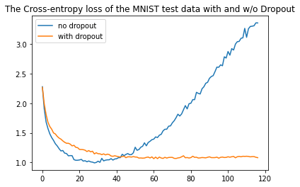
Done training.Now let's plot the test loss of both networks (with and without dropout):
import matplotlib.pyplot as plt

# plot both benchmarks
plt.plot(testing_loss, label="no dropout")
plt.plot(testing_loss_d, label="with dropout")
# make the legend on the plot
plt.legend()
plt.title("The Cross-entropy loss of the MNIST test data with and w/o Dropout")
plt.show()
Output:
Conclusion
As you can see, the test loss of the neural network without dropout started to increase after about 20 epochs, clearly overfitting. Whereas when introducing dropout, it keeps decreasing over time.
After applying the dropout technique, we notice a slight improvement. Dropout is not the sole technique that can be used to avoid overfitting. There are other techniques, such as weight decay or early stopping.
You can get the complete code for this tutorial on the Colab notebook here.
Learn also: Satellite Image Classification using TensorFlow in Python.
Happy learning ♥
Ready for more? Dive deeper into coding with our AI-powered Code Explainer. Don't miss it!
View Full Code Assist My Coding


Got a coding query or need some guidance before you comment? Check out this Python Code Assistant for expert advice and handy tips. It's like having a coding tutor right in your fingertips!