How to Build a Semantic Search Engine with FAISS and Sentence Transformers in Python

Unlock the secrets of your code with our AI-powered Code Explainer. Take a look!

Here's a sentence: "How do I make pasta at home?"

Now here's another: "Pasta carbonara is an Italian dish made with eggs, cheese, pancetta, and black pepper."

These two sentences share exactly one word: "pasta." A keyword search engine like Ctrl+F would only match them because of that single overlapping word. But you and I know they're about the same thing — cooking Italian food. The meaning is what matters, not the vocabulary.

This gap — between what words say and what they mean — is the entire reason semantic search exists. And in 2026, building one no longer requires a PhD or a cloud API key. You can run a high-quality semantic search engine entirely on your laptop, for free, with two Python libraries: Sentence Transformers for generating embeddings and FAISS for searching them at lightning speed.

In this tutorial, I'll walk you through building one from scratch. We'll embed 140 documents across 7 categories, index them with FAISS, run real semantic queries, compare against keyword search, and visualize the entire embedding space — all in under 150 lines of Python. If you've ever wondered how retrieval works in systems like ChatGPT or how RAG chatbots find relevant documents before generating answers, this is the engine that powers that retrieval step. We have a full tutorial on building a RAG chatbot that uses this exact technique with ChromaDB and LangChain.

What "Semantic Search" Actually Means

Traditional search matches tokens. You type "climate change effects" and the engine finds documents containing those exact words. This works fine until someone writes "global warming impacts" — semantically identical but lexically distinct. Keyword search sees zero overlap and returns nothing.

Semantic search matches meaning. It converts both your query and every document into a dense vector — a list of 384 numbers (or 768, or 1536) that encodes what the text is about, not just what it contains. Documents with similar meanings end up near each other in this vector space, regardless of vocabulary. When you search, the engine finds the vectors closest to your query vector and returns those documents.

This is the engine under every modern search system — Google, Spotify, Notion, ChatGPT's retrieval. And the tool that makes it possible at scale is FAISS (Facebook AI Similarity Search), an open-source library from Meta that can search billions of vectors in milliseconds.

The Stack: Sentence Transformers + FAISS

Two libraries do all the heavy lifting:

• Sentence Transformers — wraps HuggingFace transformer models to produce dense vector embeddings for sentences and paragraphs. The model we'll use (all-MiniLM-L6-v2) is 80MB, runs on CPU, and produces 384-dimensional embeddings good enough for production use. If you want to understand how transformers work under the hood, check out our guide to fine-tuning BERT for text classification — it covers the architecture that makes embeddings possible.
• FAISS — a C++ library with Python bindings that indexes vectors and finds the nearest neighbors blazingly fast. For small datasets it does exact search; for millions of vectors it switches to approximate methods that are still sub-millisecond.

Both are pure pip install — no GPU, no API keys, no Docker. Let's set them up:

pip install sentence-transformers faiss-cpu numpy rich matplotlib scikit-learn

The faiss-cpu package is all you need unless you're indexing millions of vectors. rich gives us beautiful terminal output, and we'll use scikit-learn and matplotlib for visualization.

Step 1: Prepare Your Document Corpus

Semantic search needs documents to search through. For this tutorial, I created 140 documents spread across 7 categories: Technology, Science, Cooking, Travel, Health, Business, and Arts. Each category has 20 short documents — single sentences about different topics. Here's a sample:

documents = [
    # Technology & Programming
    "Python is a high-level programming language known for its readability and simplicity",
    "Docker containers package applications with their dependencies for consistent deployment",
    "REST APIs use HTTP methods like GET, POST, PUT, and DELETE to interact with web resources",

    # Science & Nature  
    "Photosynthesis is the process by which plants convert sunlight into chemical energy",
    "Black holes are regions of spacetime where gravity is so strong that nothing can escape",
    "Plate tectonics explains how Earth's crust moves, causing earthquakes and volcanic activity",

    # Cooking & Food
    "Pasta carbonara is an Italian dish made with eggs, cheese, pancetta, and black pepper",
    "Sourdough bread uses naturally occurring wild yeast and bacteria for fermentation",
    "The Maillard reaction creates brown crusts and complex flavors when proteins are heated",

    # ... 140 documents total across 7 categories
]

The full dataset is 140 sentences — small enough to run instantly, diverse enough to demonstrate meaningful semantic clusters. In a real application, you'd replace this with thousands or millions of documents loaded from files, databases, or APIs.

Step 2: Generate Embeddings with Sentence Transformers

This is where text becomes math. The model reads each document and outputs a fixed-size vector that captures its semantic meaning:

from sentence_transformers import SentenceTransformer

# Load the model — 80MB download on first run, cached after that
model = SentenceTransformer("all-MiniLM-L6-v2")

# Encode all documents into 384-dimensional vectors
embeddings = model.encode(
    documents,
    convert_to_numpy=True,
    normalize_embeddings=True,  # L2 normalization → inner product = cosine similarity
)

print(f"Embedding shape: {embeddings.shape}")
# Output: Embedding shape: (140, 384)

Three important details here. First, normalize_embeddings=True scales every vector to unit length — this means the dot product between any two vectors becomes their cosine similarity, which is the standard way to measure semantic distance. Second, the model runs on CPU and processes our 140 documents in about 0.6 seconds. Third, the all-MiniLM-L6-v2 model is a great default: it's fast, small, and produces quality embeddings. For production, all-mpnet-base-v2 gives better quality at 2-3x the cost.

What do these embeddings actually look like? Each one is a list of 384 numbers — impossible to visualize directly, but here are the first few values of the first embedding:

[ 0.0234, -0.0891, 0.0456, -0.0123, 0.0678, ... ]  # 384 numbers total

These numbers encode the model's understanding of what the text means. Documents about cooking will have similar patterns of numbers, as will documents about science or travel — even if they use completely different vocabulary.

Step 3: Build the FAISS Index

Now we take our 140 vectors and build a searchable index. FAISS offers several index types — for this tutorial we'll use IndexFlatIP, which does exact inner product search. Since our vectors are L2-normalized, inner product equals cosine similarity:

import faiss
import numpy as np

dimension = embeddings.shape[1]  # 384

# Create an index that uses Inner Product (cosine similarity when normalized)
index = faiss.IndexFlatIP(dimension)

# Add all embeddings to the index
index.add(embeddings.astype(np.float32))

print(f"Vectors indexed: {index.ntotal}")   # 140
print(f"Dimension: {index.d}")               # 384

That's it. The index is built and ready to search. IndexFlatIP compares your query against every single vector in the index — exact but brute-force. For 140 documents this takes microseconds. For 140 million, you'd switch to IndexIVFFlat or IndexHNSWFlat, which use approximate nearest-neighbor algorithms to trade a tiny bit of accuracy for massive speed gains.

Step 4: Run Semantic Queries

The search function embeds your query the same way as the documents, then asks FAISS for the nearest neighbors:

def semantic_search(query: str, top_k: int = 5):
    """Search for documents semantically similar to the query."""
    # Embed the query (same model, same normalization)
    query_embedding = model.encode(
        [query],
        convert_to_numpy=True,
        normalize_embeddings=True,
    ).astype(np.float32)

    # Search FAISS for the k nearest neighbors
    scores, indices = index.search(query_embedding, top_k)

    # Return results with scores and documents
    results = []
    for score, idx in zip(scores[0], indices[0]):
        results.append({
            "score": float(score),
            "similarity_pct": f"{score * 100:.1f}%",
            "document": documents[idx],
        })

    return results

Now let's search. Here's what happens when you query "How do I make pasta at home?":

Query: How do I make pasta at home?

#   Score    Document
1   50.7%    Pasta carbonara is an Italian dish made with eggs, cheese, pancetta, and black pepper
2   38.5%    A roux is a mixture of flour and fat cooked together to thicken sauces and soups
3   33.3%    Mise en place means preparing and organizing all ingredients before starting to cook

Notice: the word "pasta" only appears in result #1. The other results — about roux and mise en place — don't share a single keyword with the query. Yet they're all about cooking, and the model knows it. That's semantic search.

Here's another — "What causes earthquakes and volcanic eruptions?":

Query: What causes earthquakes and volcanic eruptions?

#   Score    Document
1   71.2%    Plate tectonics explains how Earth's crust moves, causing earthquakes and volcanic activity
2   64.7%    Volcanoes form when magma from inside the Earth erupts through the crust
3   40.7%    Iceland has over 130 volcanoes and numerous geothermal hot springs used for bathing

The top result is a perfect match at 71.2%, and results 2-3 are clearly geology-related. The model understood the domain instantly.

Semantic vs Keyword: The Difference Is Dramatic

To really drive the point home, let's compare against a naive keyword approach on the same query:

def keyword_search(query: str, top_k: int = 5):
    """Simple keyword search — counts overlapping words."""
    query_words = set(query.lower().split())
    scored = []
    for i, doc in enumerate(documents):
        doc_words = set(doc.lower().split())
        overlap = len(query_words & doc_words)
        scored.append((overlap, i, doc))
    scored.sort(reverse=True)
    return scored[:top_k]

Query: "How do I create and deploy web applications?"

Keyword Search Results (word overlap):
  1. (2 matches) Plate tectonics explains how Earth's crust moves...
  2. (2 matches) The water cycle describes how water evaporates, forms clouds...
  3. (2 matches) CSS Grid and Flexbox are modern layout systems for building responsive web designs

Semantic Search Results (meaning similarity):
  1. (31.6%) Docker containers package applications with their dependencies for consistent deployment
  2. (29.9%) DevOps combines software development and IT operations to shorten the development lifecycle
  3. (26.3%) JavaScript runs in web browsers and enables interactive web pages and dynamic content

Keyword search returns plate tectonics as the #1 result — just because it contains the word "how." Semantic search returns Docker, DevOps, Kubernetes — exactly what you'd want when asking about deploying web applications. The difference isn't subtle.

Visualizing the Embedding Space

384-dimensional vectors are impossible to visualize directly, but we can use PCA (Principal Component Analysis) to project them down to 2D while preserving as much structure as possible:

from sklearn.decomposition import PCA
import matplotlib.pyplot as plt

# Reduce from 384 dimensions to 2
pca = PCA(n_components=2, random_state=42)
embeddings_2d = pca.fit_transform(embeddings)

# Color by category
categories = ["Tech", "Science", "Cooking", "Travel", "Health", "Business", "Arts"]
colors = ["#3b82f6", "#10b981", "#f59e0b", "#8b5cf6", "#ef4444", "#06b6d4", "#ec4899"]

fig, ax = plt.subplots(figsize=(14, 10))
for i, cat in enumerate(categories):
    mask = [j // 20 == i for j in range(len(documents))]
    ax.scatter(embeddings_2d[mask, 0], embeddings_2d[mask, 1],
               c=colors[i], label=cat, alpha=0.7, s=50, edgecolors='white')

ax.set_title("Document Embeddings Visualized with PCA\n384-dimensional vectors → 2D projection")
ax.legend()
plt.savefig("embedding_visualization.png", dpi=150)

Here's the result. Each dot is a document, colored by its semantic category:

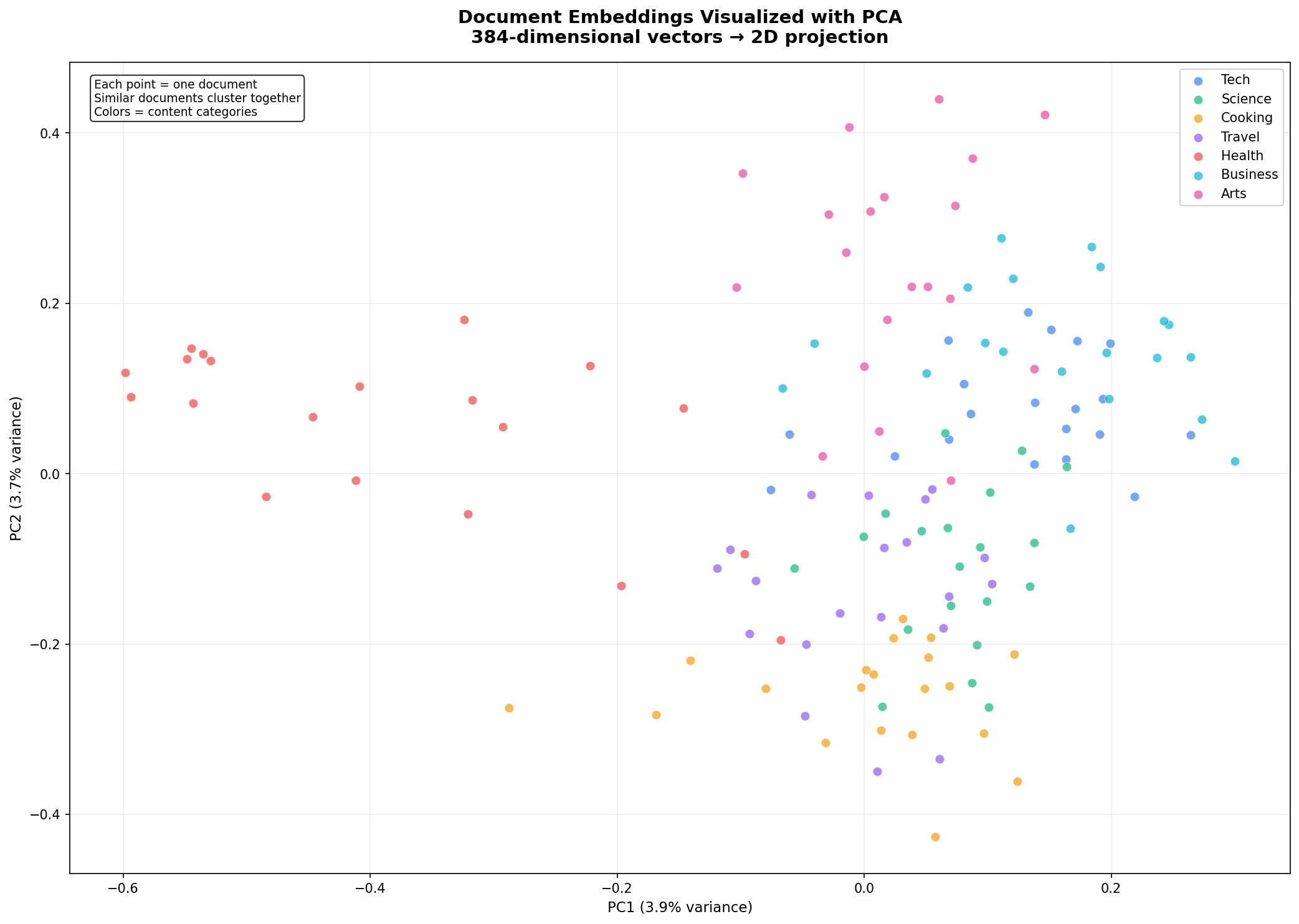
Look at how the clusters form naturally. Cooking documents (yellow) group together. Science documents (green) form their own distinct region. Tech documents (blue) cluster on the right. The model learned these semantic groupings purely from reading billions of sentences during pre-training — we never told it about our categories. It understood that "pasta carbonara" and "chocolate chip cookies" belong together, while "plate tectonics" belongs somewhere else entirely.

PC1 and PC2 together explain only about 7-8% of the total variance — normal when compressing 384 dimensions into 2. Most of the semantic structure lives in dimensions we can't see. But the visible structure is real and matches our human-labeled categories remarkably well.

Performance: How Fast Is It?

On a standard CPU, 1,000 searches across 140 documents completed in about 11 seconds — roughly 11 milliseconds per search, or 90 queries per second. This is fully brute-force (IndexFlatIP compares the query against every vector).

FAISS offers faster index types for larger datasets:

Switching index types is a one-line change — the search API stays identical.

Query-to-Cluster Mapping

As a final demonstration, here's one query from each category mapped to its top result:

Topic              Top Match                                       Score
Programming        Python is a high-level programming language     48.1%
Biology            Evolution by natural selection explains how     66.6%
Cooking            Pasta carbonara is an Italian dish made with    53.6%
Travel             New Zealand's landscape features fjords         36.3%
Fitness            Walking 10,000 steps per day is a common        51.8%
Finance            Compound interest allows investments to grow    44.4%
Art                Graffiti art transforms public walls and        56.4%

Every single query maps correctly to its semantic cluster. The model understood the domain of each query — not by matching keywords, but by understanding meaning.

Where to Go From Here

This tutorial gives you the foundation. From here, you can:

• Scale up: Replace the hardcoded document list with thousands of documents loaded from files, databases, or APIs. The pipeline stays identical.
• Add to a web app: Wrap the search engine in a FastAPI endpoint or Streamlit interface. Users type queries and get ranked results.
• Build RAG: Combine semantic retrieval with an LLM — retrieve relevant documents, inject them into a prompt, and generate answers grounded in your data. This is the architecture behind every "chat with your PDF" application. See our full guide on building a RAG chatbot that uses this exact retrieval pattern with ChromaDB and LangChain.
• Experiment with models: Swap all-MiniLM-L6-v2 for all-mpnet-base-v2 (higher quality), multi-qa-mpnet-base-dot-v1 (optimized for Q&A), or any of the 300+ models on the Sentence Transformers hub.
• Add metadata filtering: Combine FAISS vector search with traditional filters — search only within a date range, a specific category, or documents from a particular author.

Wrapping Up

You now have a working semantic search engine that runs entirely on your machine — no API keys, no cloud services, no monthly bills. The same architecture scales from 100 documents to 100 million with a one-line index change in FAISS.

What I find remarkable is how little code this requires. The heavy lifting — understanding language, converting it to vectors, searching those vectors efficiently — is all handled by two libraries. Your job is to feed them documents and ask good questions.

The complete code is below. Install the dependencies and start searching.

Further Reading:

• Sentence Transformers Documentation — model hub, training custom models, evaluation
• FAISS Wiki — index types, GPU support, performance tuning
• Building a Full-Stack RAG Chatbot with FastAPI, OpenAI, and Streamlit — practical application of semantic search with LangChain and ChromaDB

Just finished the article? Now, boost your next project with our Python Code Generator. Discover a faster, smarter way to code.

Comment panel