Unlock the secrets of your code with our AI-powered Code Explainer. Take a look!
Predicting stock prices has always been an attractive topic to investors and researchers. Investors always question if the price of a stock will rise or not; since there are many complicated financial indicators that only investors and people with good finance knowledge can understand, the stock market trend is inconsistent and looks very random to ordinary people.
Machine learning is a great opportunity for non-experts to predict accurately, gain a steady fortune, and help experts get the most informative indicators and make better predictions.
For high-quality historical stock data, consider FirstRate Data, which offers split- and dividend-adjusted intraday datasets ideal for training and backtesting models.
This tutorial aims to build a neural network in TensorFlow 2 and Keras that predicts stock market prices. More specifically, we will build a Recurrent Neural Network with LSTM cells as it is the current state-of-the-art in time series forecasting.
Alright, let's get started. First, you need to install Tensorflow 2 and some other libraries:
pip3 install tensorflow pandas numpy matplotlib yahoo_fin sklearnMore information on how you can install Tensorflow 2 here.
Once you have everything set up, open up a new Python file (or a notebook) and import the following libraries:
import tensorflow as tf
from tensorflow.keras.models import Sequential
from tensorflow.keras.layers import LSTM, Dense, Dropout, Bidirectional
from tensorflow.keras.callbacks import ModelCheckpoint, TensorBoard
from sklearn import preprocessing
from sklearn.model_selection import train_test_split
from yahoo_fin import stock_info as si
from collections import deque

import os
import numpy as np
import pandas as pd
import random
We are using yahoo_fin module, it is essentially a Python scraper that extracts finance data from the Yahoo Finance platform, so it isn't a reliable API. Feel free to use other data sources such as Alpha Vantage.
Also, we need to make sure after running our training/testing we get stable results. Setting seed will help:
# set seed, so we can get the same results after rerunning several times
np.random.seed(314)
tf.random.set_seed(314)
random.seed(314)
Learn also: How to Make a Currency Converter in Python.
Preparing the Dataset
As a first step, we need to write a function that downloads the dataset from the Internet and preprocess it:
def shuffle_in_unison(a, b):
    # shuffle two arrays in the same way
    state = np.random.get_state()
    np.random.shuffle(a)
    np.random.set_state(state)
    np.random.shuffle(b)

def load_data(ticker, n_steps=50, scale=True, shuffle=True, lookup_step=1, split_by_date=True,
                test_size=0.2, feature_columns=['adjclose', 'volume', 'open', 'high', 'low']):
    """
    Loads data from Yahoo Finance source, as well as scaling, shuffling, normalizing and splitting.
    Params:
        ticker (str/pd.DataFrame): the ticker you want to load, examples include AAPL, TESL, etc.
        n_steps (int): the historical sequence length (i.e window size) used to predict, default is 50
        scale (bool): whether to scale prices from 0 to 1, default is True
        shuffle (bool): whether to shuffle the dataset (both training & testing), default is True
        lookup_step (int): the future lookup step to predict, default is 1 (e.g next day)
        split_by_date (bool): whether we split the dataset into training/testing by date, setting it
            to False will split datasets in a random way
        test_size (float): ratio for test data, default is 0.2 (20% testing data)
        feature_columns (list): the list of features to use to feed into the model, default is everything grabbed from yahoo_fin
    """
    # see if ticker is already a loaded stock from yahoo finance
    if isinstance(ticker, str):
        # load it from yahoo_fin library
        df = si.get_data(ticker)
    elif isinstance(ticker, pd.DataFrame):
        # already loaded, use it directly
        df = ticker
    else:
        raise TypeError("ticker can be either a str or a `pd.DataFrame` instances")
    # this will contain all the elements we want to return from this function
    result = {}
    # we will also return the original dataframe itself
    result['df'] = df.copy()
    # make sure that the passed feature_columns exist in the dataframe
    for col in feature_columns:
        assert col in df.columns, f"'{col}' does not exist in the dataframe."
    # add date as a column
    if "date" not in df.columns:
        df["date"] = df.index
    if scale:
        column_scaler = {}
        # scale the data (prices) from 0 to 1
        for column in feature_columns:
            scaler = preprocessing.MinMaxScaler()
            df[column] = scaler.fit_transform(np.expand_dims(df[column].values, axis=1))
            column_scaler[column] = scaler
        # add the MinMaxScaler instances to the result returned
        result["column_scaler"] = column_scaler
    # add the target column (label) by shifting by `lookup_step`
    df['future'] = df['adjclose'].shift(-lookup_step)
    # last `lookup_step` columns contains NaN in future column
    # get them before droping NaNs
    last_sequence = np.array(df[feature_columns].tail(lookup_step))
    # drop NaNs
    df.dropna(inplace=True)
    sequence_data = []
    sequences = deque(maxlen=n_steps)
    for entry, target in zip(df[feature_columns + ["date"]].values, df['future'].values):
        sequences.append(entry)
        if len(sequences) == n_steps:
            sequence_data.append([np.array(sequences), target])
    # get the last sequence by appending the last `n_step` sequence with `lookup_step` sequence
    # for instance, if n_steps=50 and lookup_step=10, last_sequence should be of 60 (that is 50+10) length
    # this last_sequence will be used to predict future stock prices that are not available in the dataset
    last_sequence = list([s[:len(feature_columns)] for s in sequences]) + list(last_sequence)
    last_sequence = np.array(last_sequence).astype(np.float32)
    # add to result
    result['last_sequence'] = last_sequence
    # construct the X's and y's
    X, y = [], []
    for seq, target in sequence_data:
        X.append(seq)
        y.append(target)
    # convert to numpy arrays
    X = np.array(X)
    y = np.array(y)
    if split_by_date:
        # split the dataset into training & testing sets by date (not randomly splitting)
        train_samples = int((1 - test_size) * len(X))
        result["X_train"] = X[:train_samples]
        result["y_train"] = y[:train_samples]
        result["X_test"]  = X[train_samples:]
        result["y_test"]  = y[train_samples:]
        if shuffle:
            # shuffle the datasets for training (if shuffle parameter is set)
            shuffle_in_unison(result["X_train"], result["y_train"])
            shuffle_in_unison(result["X_test"], result["y_test"])
    else:
        # split the dataset randomly
        result["X_train"], result["X_test"], result["y_train"], result["y_test"] = train_test_split(X, y,
                                                                                test_size=test_size, shuffle=shuffle)
    # get the list of test set dates
    dates = result["X_test"][:, -1, -1]
    # retrieve test features from the original dataframe
    result["test_df"] = result["df"].loc[dates]
    # remove duplicated dates in the testing dataframe
    result["test_df"] = result["test_df"][~result["test_df"].index.duplicated(keep='first')]
    # remove dates from the training/testing sets & convert to float32
    result["X_train"] = result["X_train"][:, :, :len(feature_columns)].astype(np.float32)
    result["X_test"] = result["X_test"][:, :, :len(feature_columns)].astype(np.float32)
    return result
This function is long but handy, and it accepts several arguments to be as flexible as possible:
- The
tickerargument is the ticker we want to load. For instance, you can use TSLA for the Tesla stock market, AAPL for Apple, and so on. It can also be a pandas Dataframe with the condition it includes the columns infeature_columnsand date as an index. n_stepsinteger indicates the historical sequence length we want to use; some people call it the window size, recall that we are going to use a recurrent neural network, we need to feed into the network a sequence data, choosing 50 means that we will use 50 days of stock prices to predict the next lookup time step.scaleis a boolean variable that indicates whether to scale prices from 0 to 1; we will set this toTrueas scaling high values from 0 to 1 will help the neural network to learn much faster and more effectively.lookup_stepis the future lookup step to predict, the default is set to 1 (e.g., next day). 15 means the next 15 days, and so on.split_by_dateis a boolean that indicates whether we split our training and testing sets by date. Setting it toFalsemeans we randomly split the data into training and testing using sklearn'strain_test_split()function. If it'sTrue(the default), we split the data in date order.
We will use all the features available in this dataset: open, high, low, volume, and adjusted close. Please check this tutorial to learn more about what these indicators are.
The above function does the following:
- First, it loads the dataset using stock_info.get_data() function in yahoo_fin module.
- It adds the
"date"column from the index if it doesn't exist, this will help us later to get the features of the testing set. - If the scale argument is passed as True, it will scale all the prices from 0 to 1 (including the volume) using sklearn's MinMaxScaler class. Note that each column has its own scaler.
- It then adds the future column, which indicates the target values (the labels to predict, or the y's) by shifting the adjusted close column by lookup_step.
- After that, it shuffles and splits the data into training and testing sets and finally returns the result.
To understand the code even better, I highly suggest you manually print the output variable (result) and see how the features and labels are made.
Learn also: How to Make a Speech Emotion Recognizer Using Python And Scikit-learn.
Model Creation
Now that we have a proper function to load and prepare the dataset, we need another core function to build our model:
def create_model(sequence_length, n_features, units=256, cell=LSTM, n_layers=2, dropout=0.3,
                loss="mean_absolute_error", optimizer="rmsprop", bidirectional=False):
    model = Sequential()
    for i in range(n_layers):
        if i == 0:
            # first layer
            if bidirectional:
                model.add(Bidirectional(cell(units, return_sequences=True), batch_input_shape=(None, sequence_length, n_features)))
            else:
                model.add(cell(units, return_sequences=True, batch_input_shape=(None, sequence_length, n_features)))
        elif i == n_layers - 1:
            # last layer
            if bidirectional:
                model.add(Bidirectional(cell(units, return_sequences=False)))
            else:
                model.add(cell(units, return_sequences=False))
        else:
            # hidden layers
            if bidirectional:
                model.add(Bidirectional(cell(units, return_sequences=True)))
            else:
                model.add(cell(units, return_sequences=True))
        # add dropout after each layer
        model.add(Dropout(dropout))
    model.add(Dense(1, activation="linear"))
    model.compile(loss=loss, metrics=["mean_absolute_error"], optimizer=optimizer)
    return model
Again, this function is flexible too, and you can change the number of layers, dropout rate, the RNN cell, loss, and the optimizer used to compile the model.
The above function constructs an RNN with a dense layer as an output layer with one neuron. This model requires a sequence of features of sequence_length (in this case, we will pass 50 or 100) consecutive time steps (which are days in this dataset) and outputs a single value which indicates the price of the next time step.
It also accepts n_features as an argument, which is the number of features we will pass on each sequence, in our case, we'll pass adjclose, open, high, low and volume columns (i.e 5 features).
You can tweak the default parameters as you wish, n_layers is the number of RNN layers you want to stack, dropout is the dropout rate after each RNN layer, units are the number of RNN cell units (whether it is LSTM, SimpleRNN, or GRU), bidirectional is a boolean that indicates whether to use bidirectional RNNs, experiment with those!
Training the Model
Now that we have all the core functions ready, let's train our model, but before we do that, let's initialize all our parameters (so you can edit them later on your needs):
import os
import time
from tensorflow.keras.layers import LSTM

# Window size or the sequence length
N_STEPS = 50
# Lookup step, 1 is the next day
LOOKUP_STEP = 15
# whether to scale feature columns & output price as well
SCALE = True
scale_str = f"sc-{int(SCALE)}"
# whether to shuffle the dataset
SHUFFLE = True
shuffle_str = f"sh-{int(SHUFFLE)}"
# whether to split the training/testing set by date
SPLIT_BY_DATE = False
split_by_date_str = f"sbd-{int(SPLIT_BY_DATE)}"
# test ratio size, 0.2 is 20%
TEST_SIZE = 0.2
# features to use
FEATURE_COLUMNS = ["adjclose", "volume", "open", "high", "low"]
# date now
date_now = time.strftime("%Y-%m-%d")
### model parameters
N_LAYERS = 2
# LSTM cell
CELL = LSTM
# 256 LSTM neurons
UNITS = 256
# 40% dropout
DROPOUT = 0.4
# whether to use bidirectional RNNs
BIDIRECTIONAL = False
### training parameters
# mean absolute error loss
# LOSS = "mae"
# huber loss
LOSS = "huber_loss"
OPTIMIZER = "adam"
BATCH_SIZE = 64
EPOCHS = 500
# Amazon stock market
ticker = "AMZN"
ticker_data_filename = os.path.join("data", f"{ticker}_{date_now}.csv")
# model name to save, making it as unique as possible based on parameters
model_name = f"{date_now}_{ticker}-{shuffle_str}-{scale_str}-{split_by_date_str}-\
{LOSS}-{OPTIMIZER}-{CELL.__name__}-seq-{N_STEPS}-step-{LOOKUP_STEP}-layers-{N_LAYERS}-units-{UNITS}"
if BIDIRECTIONAL:
    model_name += "-b"
So the above code is all about defining all the hyperparameters we gonna use; we explained some of them while we didn't explain the others:
TEST_SIZE: The testing set rate. For instance,0.2means20%of the total dataset.FEATURE_COLUMNS: The features we gonna use to predict the next price value.N_LAYERS: Number of RNN layers to use.CELL: RNN cell to use, default is LSTM.UNITS: Number ofcellunits.DROPOUT: The dropout rate is the probability of not training a given node in a layer, where 0.0 means no dropout at all. This regularization can help the model not overfit our training data. Check this tutorial for more information about dropout regularization.BIDIRECTIONAL: Whether to use bidirectional recurrent neural networks.LOSS: Loss function to use for this regression problem, we're using Huber loss, you can use mean absolute error (mae) or mean squared error (mse) as well.OPTIMIZER: Optimization algorithm to use, defaulting to Adam.BATCH_SIZE: The number of data samples to use on each training iteration.EPOCHS: The number of times the learning algorithm will pass through the entire training dataset, we used 500 here, but try to increase it further.
Feel free to experiment with these values to get better results than mine.
Alright, let's make sure the results, logs, and data folders exist before we train:
# create these folders if they does not exist
if not os.path.isdir("results"):
    os.mkdir("results")
if not os.path.isdir("logs"):
    os.mkdir("logs")
if not os.path.isdir("data"):
    os.mkdir("data")
Finally, let's call the above functions to train our model:
# load the data
data = load_data(ticker, N_STEPS, scale=SCALE, split_by_date=SPLIT_BY_DATE,
                shuffle=SHUFFLE, lookup_step=LOOKUP_STEP, test_size=TEST_SIZE,
                feature_columns=FEATURE_COLUMNS)
# save the dataframe
data["df"].to_csv(ticker_data_filename)
# construct the model
model = create_model(N_STEPS, len(FEATURE_COLUMNS), loss=LOSS, units=UNITS, cell=CELL, n_layers=N_LAYERS,
                    dropout=DROPOUT, optimizer=OPTIMIZER, bidirectional=BIDIRECTIONAL)
# some tensorflow callbacks
checkpointer = ModelCheckpoint(os.path.join("results", model_name + ".h5"), save_weights_only=True, save_best_only=True, verbose=1)
tensorboard = TensorBoard(log_dir=os.path.join("logs", model_name))
# train the model and save the weights whenever we see
# a new optimal model using ModelCheckpoint
history = model.fit(data["X_train"], data["y_train"],
                    batch_size=BATCH_SIZE,
                    epochs=EPOCHS,
                    validation_data=(data["X_test"], data["y_test"]),
                    callbacks=[checkpointer, tensorboard],
                    verbose=1)
We used ModelCheckpoint, which saves our model in each epoch during the training. We also used TensorBoard to visualize the model performance in the training process.
After running the above block of code, it will train the model for 500 epochs (as we set previously), so it will take some time. Here are the first output lines:
Train on 4696 samples, validate on 1175 samples
Epoch 1/500
4608/4696 [============================>.] - ETA: 0s - loss: 0.0011 - mean_absolute_error: 0.0211
Epoch 00001: val_loss improved from inf to 0.00011, saving model to results\2020-12-11_AMZN-sh-1-sc-1-sbd-0-huber_loss-adam-LSTM-seq-50-step-15-layers-2-units-256.h5
4696/4696 [==============================] - 7s 2ms/sample - loss: 0.0011 - mean_absolute_error: 0.0211 - val_loss: 1.0943e-04 - val_mean_absolute_error: 0.0071
Epoch 2/500
4544/4696 [============================>.] - ETA: 0s - loss: 4.3212e-04 - mean_absolute_error: 0.0146
Epoch 00002: val_loss did not improve from 0.00011
4696/4696 [==============================] - 2s 411us/sample - loss: 4.2579e-04 - mean_absolute_error: 0.0144 - val_loss: 1.5914e-04 - val_mean_absolute_error: 0.0104
After the training ends (or during the training), try to run tensorboard using this command:
tensorboard --logdir="logs"Now, this will start a local HTTP server at localhost:6006; after going to the browser, you'll see something similar to this:
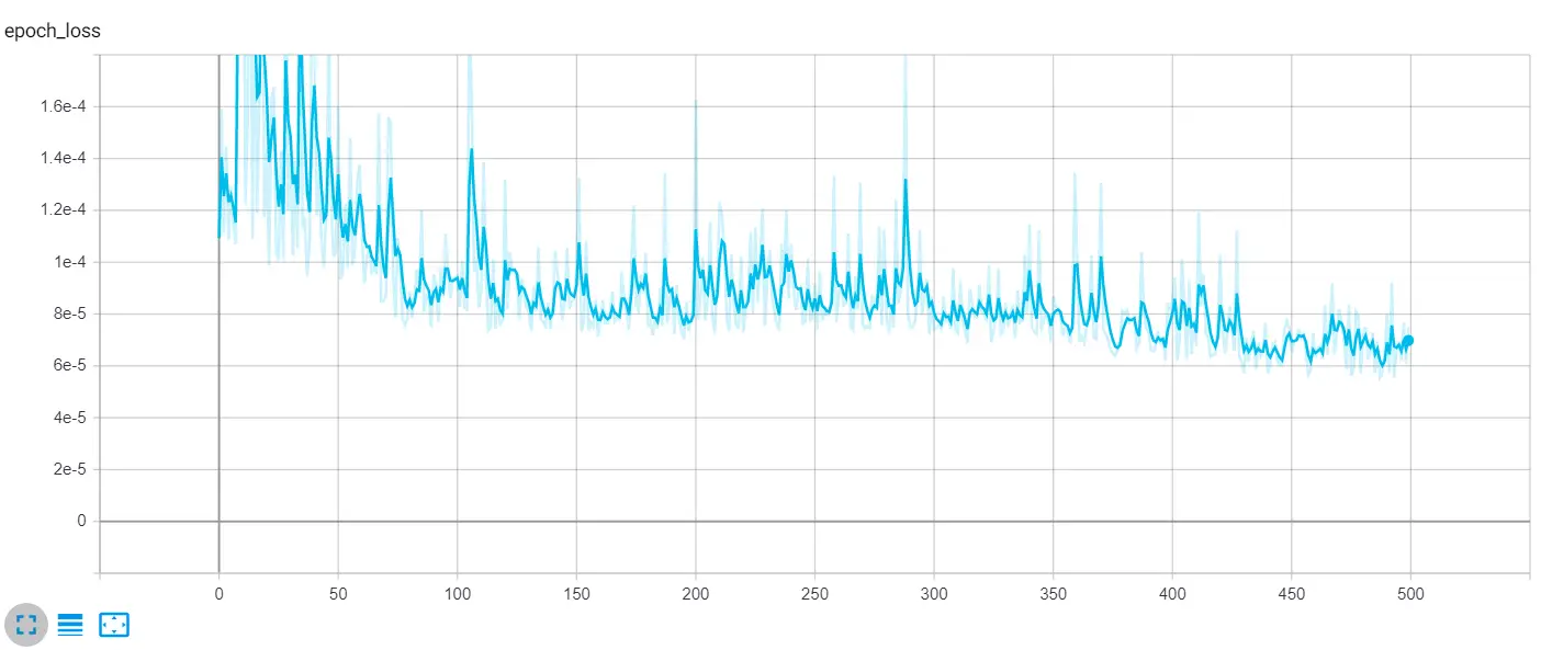
The loss is Huber loss as specified in the LOSS parameter (you can always change it to mean absolute error or mean squared error), the curve is the validation loss. As you can see, it is significantly decreasing over time. You can also increase the number of epochs to get much better results.
Testing the Model
Now that we've trained our model, let's evaluate it and see how it's doing on the testing set. The below function takes a pandas Dataframe and plots the true and predicted prices in the same plot using matplotlib. We'll use it later:
import matplotlib.pyplot as plt

def plot_graph(test_df):
    """
    This function plots true close price along with predicted close price
    with blue and red colors respectively
    """
    plt.plot(test_df[f'true_adjclose_{LOOKUP_STEP}'], c='b')
    plt.plot(test_df[f'adjclose_{LOOKUP_STEP}'], c='r')
    plt.xlabel("Days")
    plt.ylabel("Price")
    plt.legend(["Actual Price", "Predicted Price"])
    plt.show()
The below function takes the model and the data that was returned by create_model() and load_data() functions respectively, and constructs a dataframe that includes the predicted adjclose along with true future adjclose, as well as calculating buy and sell profit. We'll see it in action in a moment:
def get_final_df(model, data):
    """
    This function takes the `model` and `data` dict to
    construct a final dataframe that includes the features along
    with true and predicted prices of the testing dataset
    """
    # if predicted future price is higher than the current,
    # then calculate the true future price minus the current price, to get the buy profit
    buy_profit  = lambda current, pred_future, true_future: true_future - current if pred_future > current else 0
    # if the predicted future price is lower than the current price,
    # then subtract the true future price from the current price
    sell_profit = lambda current, pred_future, true_future: current - true_future if pred_future < current else 0
    X_test = data["X_test"]
    y_test = data["y_test"]
    # perform prediction and get prices
    y_pred = model.predict(X_test)
    if SCALE:
        y_test = np.squeeze(data["column_scaler"]["adjclose"].inverse_transform(np.expand_dims(y_test, axis=0)))
        y_pred = np.squeeze(data["column_scaler"]["adjclose"].inverse_transform(y_pred))
    test_df = data["test_df"]
    # add predicted future prices to the dataframe
    test_df[f"adjclose_{LOOKUP_STEP}"] = y_pred
    # add true future prices to the dataframe
    test_df[f"true_adjclose_{LOOKUP_STEP}"] = y_test
    # sort the dataframe by date
    test_df.sort_index(inplace=True)
    final_df = test_df
    # add the buy profit column
    final_df["buy_profit"] = list(map(buy_profit,
                                    final_df["adjclose"],
                                    final_df[f"adjclose_{LOOKUP_STEP}"],
                                    final_df[f"true_adjclose_{LOOKUP_STEP}"])
                                    # since we don't have profit for last sequence, add 0's
                                    )
    # add the sell profit column
    final_df["sell_profit"] = list(map(sell_profit,
                                    final_df["adjclose"],
                                    final_df[f"adjclose_{LOOKUP_STEP}"],
                                    final_df[f"true_adjclose_{LOOKUP_STEP}"])
                                    # since we don't have profit for last sequence, add 0's
                                    )
    return final_df
The last function we going to define is the one that's responsible for predicting the next future price:
def predict(model, data):
    # retrieve the last sequence from data
    last_sequence = data["last_sequence"][-N_STEPS:]
    # expand dimension
    last_sequence = np.expand_dims(last_sequence, axis=0)
    # get the prediction (scaled from 0 to 1)
    prediction = model.predict(last_sequence)
    # get the price (by inverting the scaling)
    if SCALE:
        predicted_price = data["column_scaler"]["adjclose"].inverse_transform(prediction)[0][0]
    else:
        predicted_price = prediction[0][0]
    return predicted_price
Now that we have the necessary functions for evaluating our model, let's load the optimal weights and proceed with evaluation:
# load optimal model weights from results folder
model_path = os.path.join("results", model_name) + ".h5"
model.load_weights(model_path)
Calculating loss and mean absolute error using model.evaluate() method:
# evaluate the model
loss, mae = model.evaluate(data["X_test"], data["y_test"], verbose=0)
# calculate the mean absolute error (inverse scaling)
if SCALE:
    mean_absolute_error = data["column_scaler"]["adjclose"].inverse_transform([[mae]])[0][0]
else:
    mean_absolute_error = mae
We also take scaled output values into consideration, so we use the inverse_transform() method from the MinMaxScaler we defined in the load_data() function earlier if the SCALE parameter was set to True.
Now let's call the get_final_df() function we defined earlier to construct our testing set dataframe:
# get the final dataframe for the testing set
final_df = get_final_df(model, data)
Also, let's use predict() function to get the future price:
# predict the future price
future_price = predict(model, data)
The below code calculates the accuracy score by counting the number of positive profits (in both buy profit and sell profit):
# we calculate the accuracy by counting the number of positive profits
accuracy_score = (len(final_df[final_df['sell_profit'] > 0]) + len(final_df[final_df['buy_profit'] > 0])) / len(final_df)
# calculating total buy & sell profit
total_buy_profit  = final_df["buy_profit"].sum()
total_sell_profit = final_df["sell_profit"].sum()
# total profit by adding sell & buy together
total_profit = total_buy_profit + total_sell_profit
# dividing total profit by number of testing samples (number of trades)
profit_per_trade = total_profit / len(final_df)
We also calculate profit per trade which is essentially the total profit divided by the number of testing samples. Printing all the previously calculated metrics:
# printing metrics
print(f"Future price after {LOOKUP_STEP} days is {future_price:.2f}$")
print(f"{LOSS} loss:", loss)
print("Mean Absolute Error:", mean_absolute_error)
print("Accuracy score:", accuracy_score)
print("Total buy profit:", total_buy_profit)
print("Total sell profit:", total_sell_profit)
print("Total profit:", total_profit)
print("Profit per trade:", profit_per_trade)
Output:
Future price after 15 days is 3232.24$
huber_loss loss: 8.655239071231335e-05
Mean Absolute Error: 24.113272707281315
Accuracy score: 0.5884808013355592
Total buy profit: 10710.308540344238
Total sell profit: 2095.779877185823
Total profit: 12806.088417530062
Profit per trade: 10.68955627506683
Great, the model says after 15 days that the price of AMZN will be 3232.24$, that's interesting!
Below is the meaning of the main metrics:
- Mean absolute error: we get about 20 as error, which means, on average, the model predictions are far by over 20$ to the true prices; this will vary from
tickerto another, as prices get larger, the error will increase as well. As a result, you should only compare your models using this metric when the ticker is stable (e.g., AMZN). - Buy/Sell profit: This is the profit we get if we opened trades on all the testing samples, we calculated these on
get_final_df()function. - Total profit: This is simply the sum of buy and sell profits.
- Profit per trade: The total profit divided by the total number of testing samples.
- Accuracy score: This is the score of how accurate our predictions are. This calculation is based on the positive profits from all the trades from the testing samples.
I invite you to tweak the parameters or change the LOOKUP_STEP to get the best possible error, accuracy, and profit!
Now let's plot our graph that shows the actual and predicted prices:
# plot true/pred prices graph
plot_graph(final_df)
Result:
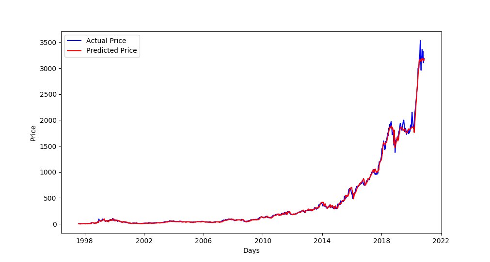 Excellent, as you can see, the blue curve is the actual test set, and the red curve is the predicted prices! Notice that the stock price has recently been increasing, as we predicted.
Since we set SPLIT_BY_DATE to False, this plot shows the prices of the testing set spread on our whole dataset along with corresponding predicted prices (which explains the testing set starts before 1998).
If we set SPLIT_BY_DATE to True, then the testing set will be the last TEST_SIZE percentage of the total dataset (For instance, if we have data from 1997 to 2020, and TEST_SIZE is 0.2, then testing samples will range from about 2016 to 2020).
Finally, let's print the last ten rows of our final dataframe, so you can see what it looks like:
print(final_df.tail(10))
# save the final dataframe to csv-results folder
csv_results_folder = "csv-results"
if not os.path.isdir(csv_results_folder):
    os.mkdir(csv_results_folder)
csv_filename = os.path.join(csv_results_folder, model_name + ".csv")
final_df.to_csv(csv_filename)
We also saved the dataframe in csv-results folder, there is the output:
            open        high        low         close       adjclose    volume  ticker  adjclose_15 true_adjclose_15  buy_profit    sell_profit
2021-03-10	3098.449951	3116.459961	3030.050049	3057.639893	3057.639893	3012500	AMZN	3239.598633	3094.080078       36.440186     0.000000
2021-03-11	3104.010010	3131.780029	3082.929932	3113.590088	3113.590088	2776400	AMZN	3238.842773	3161.000000       47.409912     0.000000
2021-03-12	3075.000000	3098.979980	3045.500000	3089.489990	3089.489990	2421900	AMZN	3238.662598	3226.729980       137.239990    0.000000
2021-03-15	3074.570068	3082.239990	3032.090088	3081.679932	3081.679932	2913600	AMZN	3238.824219	3223.820068       142.140137    0.000000
2021-03-17	3073.219971	3173.050049	3070.219971	3135.729980	3135.729980	3118600	AMZN	3238.115234	3299.300049       163.570068    0.000000
2021-03-18	3101.000000	3116.629883	3025.000000	3027.989990	3027.989990	3649600	AMZN	3238.491943	3372.199951       344.209961    0.000000
2021-03-25	3072.989990	3109.780029	3037.139893	3046.260010	3046.260010	3563500	AMZN	3238.083740	3399.439941       353.179932    0.000000
2021-04-15	3371.000000	3397.000000	3352.000000	3379.090088	3379.090088	3233600	AMZN	3223.817627	3306.370117       0.000000      72.719971
2021-04-23	3319.100098	3375.000000	3308.500000	3340.879883	3340.879883	3192800	AMZN	3226.480957	3222.899902       0.000000      117.979980
2021-05-03	3484.729980	3486.649902	3372.699951	3386.489990	3386.489990	5875500	AMZN	3217.589844	3244.989990       0.000000      141.500000
The dataframe has the following columns:
- Our testing set features (open, high, low, close, adjclose, and volume columns).
adjclose_15: is the predictedadjcloseprice after 15 days (sinceLOOKUP_STEPis set to 15) using our trained model.true_adjclose_15: is the trueadjcloseprice after 15 days; we get that by shifting our testing dataset.buy_profit: This is the profit we get if we bought the stock at that date. A negative profit means we made a loss (it should be a sell trade, and we made a buy).sell_profit: This is the profit we get if we sell the stock at that date.
Conclusion
Alright, that's it for this tutorial. You can tweak the parameters and see how you can improve the model performance, try to train on more epochs, say 700 or even more, increase or decrease the BATCH_SIZE and see if it does change for the better, or play around with N_STEPS and LOOKUP_STEPS and see which combination works best.
You can also change the model parameters by increasing the number of layers or LSTM units or even trying the GRU cell instead of LSTM.
Note that there are other features and indicators to use, to improve the prediction, it is often known to use some other information like features, such as technical indicators, the company product innovation, interest rate, exchange rate, public policy, the web, and financial news and even the number of employees!
I encourage you to change the model architecture, try to use CNNs or Seq2Seq models, or even add bidirectional LSTMs to this existing model (setting BIDIRECTIONAL to True), see if you can improve it!
Also, use different stock markets, check the Yahoo Finance page, and see which one you actually want!
To check the full code, I encourage you to use either the complete notebook or the full code split into different Python files.
Read also: How to Perform Voice Gender Recognition using TensorFlow in Python.
Happy Training ♥
Let our Code Converter simplify your multi-language projects. It's like having a coding translator at your fingertips. Don't miss out!
View Full Code Create Code for Me


Got a coding query or need some guidance before you comment? Check out this Python Code Assistant for expert advice and handy tips. It's like having a coding tutor right in your fingertips!