Unlock the secrets of your code with our AI-powered Code Explainer. Take a look!
SIFT stands for Scale Invariant Feature Transform, it is a feature extraction method (among others, such as HOG feature extraction) where image content is transformed into local feature coordinates that are invariant to translation, scale and other image transformations.
In this tutorial, you will learn the theory behind SIFT as well as how to implement it in Python using the OpenCV library.
Below are the advantages of SIFT:
- Locality: Features are local; robust to occlusion and clutter.
- Distinctiveness: Individual features extracted can be matched to a large dataset of objects.
- Quantity: Using SIFT, we can extract many features from small objects.
- Efficiency: SIFT is close to real-time performance.
These are the high-level details of SIFT:
- Scale-space Extrema Detection: Identify locations and scales that can be repeatedly assigned under different views of the same scene or object.
- Keypoint Localization: Fit a model to determine the location and scale of features, selecting key points based on a measure of stability.
- Orientation Assignment: Compute best orientation(s) for each keypoint region.
- Keypoint Description: Use local image gradients at the selected scale and rotation to describe each keypoint region.
Scale-space Extrema Detection
In the first step, we identify locations and scales that can be repeatedly assigned under different views of the same object or scene. For the identification, we will search for stable features across multiple scales using a continuous function of scale using the Gaussian function.
The scale-space of an image is a function L(x, y, a) that is produced from the convolution of a Gaussian kernel (at different scales) with the input image.
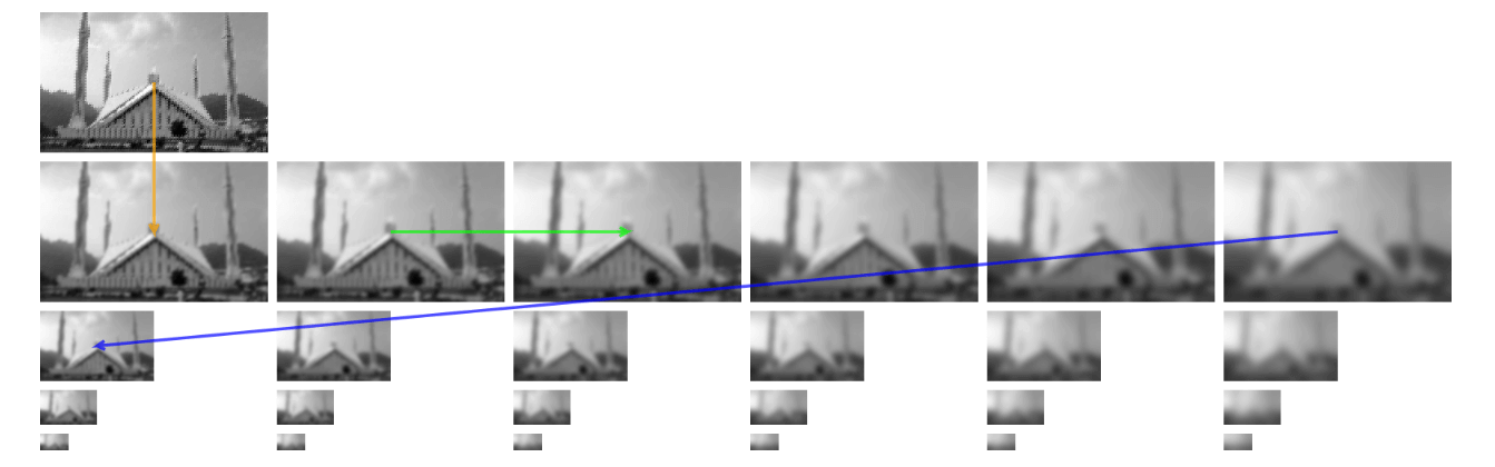
In each octave, the initial image is repeatedly convolved with Gaussians to produce a set of scale-space images. At each level, the image is smoothed and reduced in size. After each octave, the Gaussian image is down-sampled by a factor of 2 to produce an image 1/4 the size to start the next level. The adjacent Gaussians are subtracted to produce the DoG (Difference of Gaussians).
For creating the first octave, a gaussian filter is applied to an input image with different values of sigma, then for the 2nd and upcoming octaves, the image is first down-sampled by a factor of 2 then applied Gaussian filters with different values.
The sigma values are as follows.
- Octave 1 uses a scale of σ.
- Octave 2 uses a scale of 2σ.
- And so on.
The following image shows four octaves and each octave contains six images:
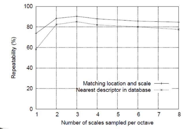
A question comes around about how many scales per octave? Research shows that there should be 4 scales per octave:
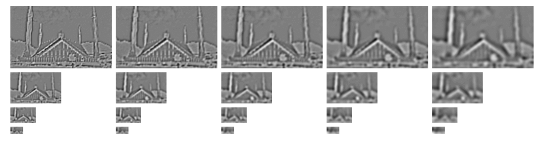
Then, two consecutive images in the octave are subtracted to obtain the difference of Gaussian.
Keypoint Localization
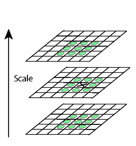
After taking the difference of Gaussian, we need to detect the maxima and minima in the scale space by comparing a pixel (x) with 26 pixels in the current and adjacent scale. Each point is compared to its 8 neighbors in the current image and 9 neighbors each in the scales above and below.
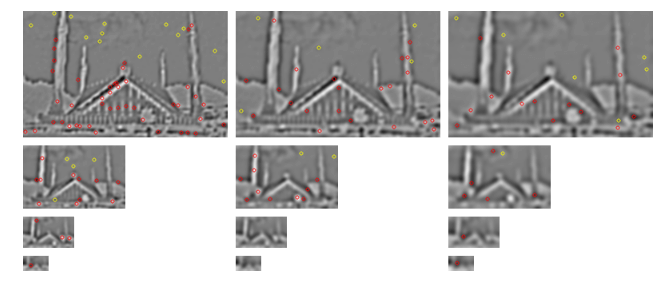
The following are the extrema points found in our example image:
Related: Mastering YOLO: Build an Automatic Number Plate Recognition System with OpenCV in Python.
Orientation Assignment
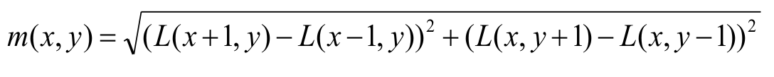
Orientation assignments are done to achieve rotation invariance. The gradient magnitude and direction calculations are done for every pixel in a neighboring region around the key point in the Gaussian-blurred image.
The magnitude represents the intensity of the pixel and the orientation gives the direction for the same.
The formula used for gradient magnitude is:
The formula for direction calculation is:
![]()
Now we need to look at the orientation of each point. weights are also assigned with the direction. The arrow in the blue square below has an approximately 90-degree angle, and its length shows how much it counts.
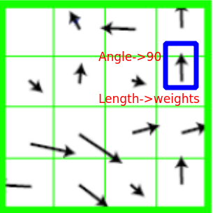
A histogram is formed by quantizing the orientations into 36 bins, with each bin covering 10 degrees. The histogram will show us how many pixels have a certain angle. For example, how many pixels have 36 degrees angle?
![]()
Keypoint Description
At this point, each key point has a location, scale, and orientation. Now, we need to compute a descriptor for that. We need to use the normalized region around the key point. We will first take a 16×16 neighborhood around the key point. This 16×16 block is further divided into 4×4 sub-blocks and for each of these sub-blocks, we generate the histogram using magnitude and orientation.
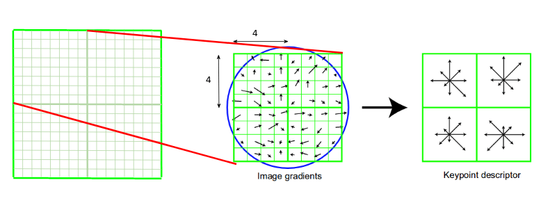
Concatenate 16 histograms in one long vector of 128 dimensions. 4x4 times 8 directions gives a vector of 128 values.
Read also: How to Apply HOG Feature Extraction in Python.
Python Implementation
Now you hopefully understand the theory behind SIFT, let's dive into the Python code using OpenCV. First, let's install a specific version of OpenCV which implements SIFT:
pip3 install numpy opencv-python==3.4.2.16 opencv-contrib-python==3.4.2.16Open up a new Python file and follow along, I'm gonna operate on this table that contains a specific book (get it here):
import cv2

# reading the image
img = cv2.imread('table.jpg')
# convert to greyscale
gray = cv2.cvtColor(img, cv2.COLOR_BGR2GRAY)
The above code loads the image and converts it to grayscale, let's create the SIFT feature extractor object:
# create SIFT feature extractor
sift = cv2.xfeatures2d.SIFT_create()
To detect the key points and descriptors, we simply pass the image to detectAndCompute() method:
# detect features from the image
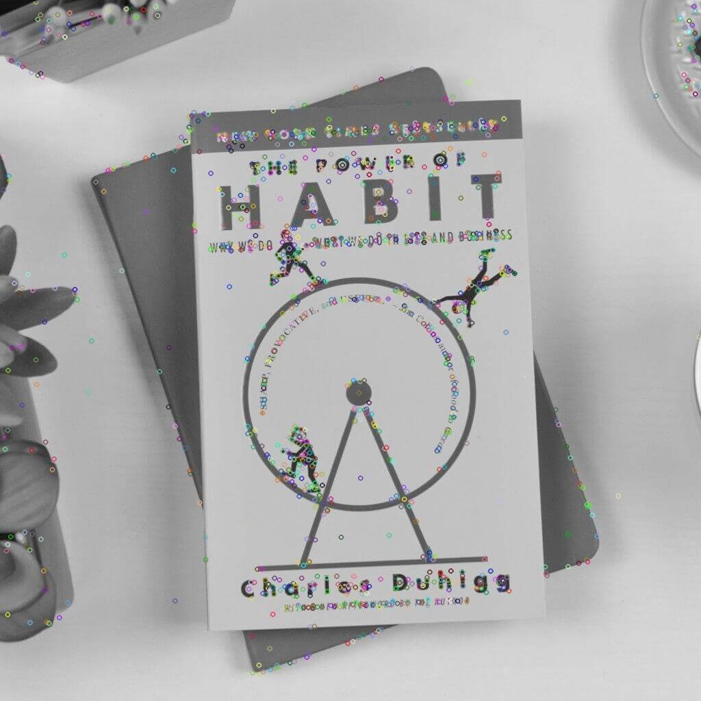
keypoints, descriptors = sift.detectAndCompute(img, None)Finally, let's draw the key points, show and save the image:
# draw the detected key points
sift_image = cv2.drawKeypoints(gray, keypoints, img)
# show the image
cv2.imshow('image', sift_image)
# save the image
cv2.imwrite("table-sift.jpg", sift_image)
cv2.waitKey(0)
cv2.destroyAllWindows()
Here is the resulting image:
These SIFT feature points are useful for many use cases, here are some:
- Image alignment (homography, fundamental matrix)
- Feature matching
- 3D reconstruction
- Motion tracking
- Object recognition
- Indexing and database retrieval
- Robot navigation
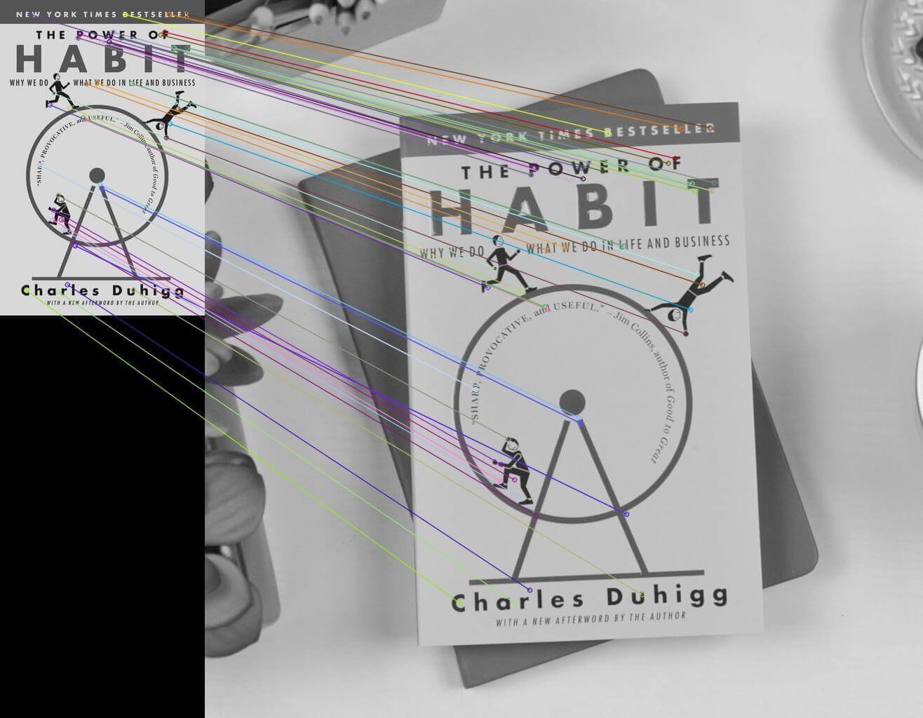
To make a real-world use in this demonstration, we're picking feature matching, let's use OpenCV to match 2 images of the same object from different angles (you can get the images in this GitHub repository):
import cv2

# read the images
img1 = cv2.imread('book.jpg')
img2 = cv2.imread('table.jpg')
# convert images to grayscale
img1 = cv2.cvtColor(img1, cv2.COLOR_BGR2GRAY)
img2 = cv2.cvtColor(img2, cv2.COLOR_BGR2GRAY)
# create SIFT object
sift = cv2.xfeatures2d.SIFT_create()
# detect SIFT features in both images
keypoints_1, descriptors_1 = sift.detectAndCompute(img1,None)
keypoints_2, descriptors_2 = sift.detectAndCompute(img2,None)
Now that we have key points and descriptors of both images, let's make a matcher to match the descriptors:
# create feature matcher
bf = cv2.BFMatcher(cv2.NORM_L1, crossCheck=True)
# match descriptors of both images
matches = bf.match(descriptors_1,descriptors_2)
Let's sort the matches by distance and draw the first 50 matches:
# sort matches by distance
matches = sorted(matches, key = lambda x:x.distance)
# draw first 50 matches
matched_img = cv2.drawMatches(img1, keypoints_1, img2, keypoints_2, matches[:50], img2, flags=2)
Finally, showing and saving the image:
# show the image
cv2.imshow('image', matched_img)
# save the image
cv2.imwrite("matched_images.jpg", matched_img)
cv2.waitKey(0)
cv2.destroyAllWindows()
Output:
Conclusion
Alright, in this tutorial, we've covered the basics of SIFT, I suggest you read the original paper for more detailed information.
Also, OpenCV uses the default parameters of SIFT in cv2.xfeatures2d.SIFT_create() method, you can change the number of features to retain (nfeatures), nOctaveLayers, sigma and more. Type help(cv2.xfeatures2d.SIFT_create) for more information.
Learn also: How to Detect Shapes in Images in Python using OpenCV.
Happy learning ♥
Want to code smarter? Our Python Code Assistant is waiting to help you. Try it now!
View Full Code Generate Python Code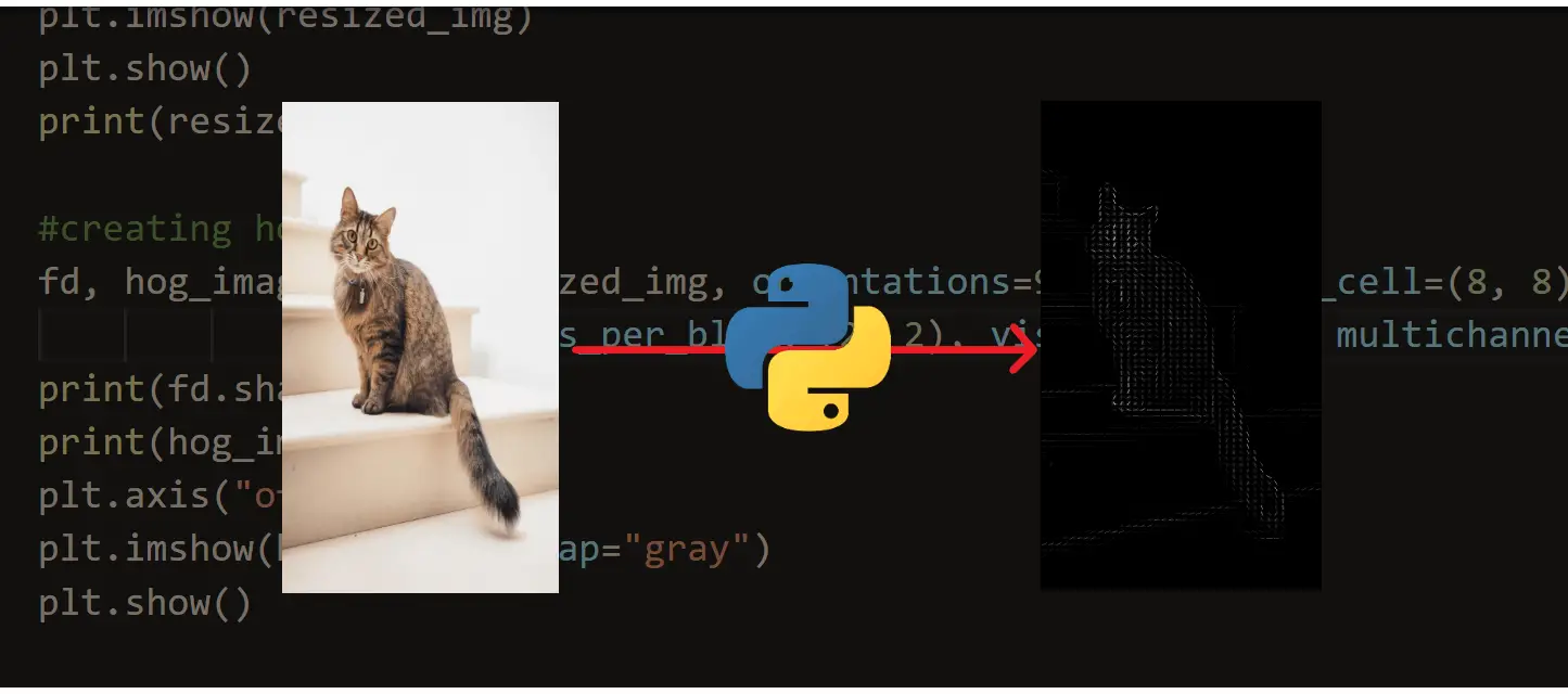


Got a coding query or need some guidance before you comment? Check out this Python Code Assistant for expert advice and handy tips. It's like having a coding tutor right in your fingertips!